Page 155 - Computational Statistics Handbook with MATLAB

142 Computational Statistics Handbook with MATLAB

Example 5.14
We generate bivariate standard normal random variables and use them to
illustrate how to get the bivariate density histogram. We use the optimal bin
width for data generated from a standard bivariate normal given in Scott
[1992]. We postpone discussion of the optimal bin width and how to obtain it
until Chapter 8. A scatterplot of the data and the resulting histogram are
shown in Figure 5.22.
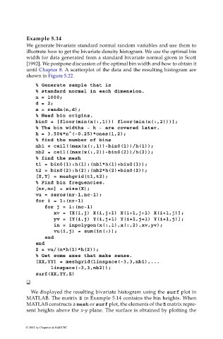
% Generate sample that is
% standard normal in each dimension.
n = 1000;
d = 2;
x = randn(n,d);
% Need bin origins.
bin0 = [floor(min(x(:,1))) floor(min(x(:,2)))];
% The bin widths - h - are covered later.
h = 3.504*n^(-0.25)*ones(1,2);
% find the number of bins
nb1 = ceil((max(x(:,1))-bin0(1))/h(1));
nb2 = ceil((max(x(:,2))-bin0(2))/h(2));
% find the mesh
t1 = bin0(1):h(1):(nb1*h(1)+bin0(1));
t2 = bin0(2):h(2):(nb2*h(2)+bin0(2));
[X,Y] = meshgrid(t1,t2);
% Find bin frequencies.
[nr,nc] = size(X);
vu = zeros(nr-1,nc-1);
for i = 1:(nr-1)
for j = 1:(nc-1)
xv = [X(i,j) X(i,j+1) X(i+1,j+1) X(i+1,j)];
yv = [Y(i,j) Y(i,j+1) Y(i+1,j+1) Y(i+1,j)];
in = inpolygon(x(:,1),x(:,2),xv,yv);
vu(i,j) = sum(in(:));
end
end
Z = vu/(n*h(1)*h(2));
% Get some axes that make sense.
[XX,YY] = meshgrid(linspace(-3,3,nb1),...
linspace(-3,3,nb2));
surf(XX,YY,Z)

We displayed the resulting bivariate histogram using the surf plot in
MATLAB. The matrix Z in Example 5.14 contains the bin heights. When
MATLAB constructs a mesh or surf plot, the elements of the Z matrix repre-
sent heights above the x-y plane. The surface is obtained by plotting the

© 2002 by Chapman & Hall/CRC