Page 154 - Computational Statistics Handbook with MATLAB

Chapter 5: Exploratory Data Analysis 141

10

5

0

−5

−10
2 3
2
0 1
0
−2 −2 −1
−3
FI F U URE G 5.2 RE 5.2 1 1
IG
GU
F F II GU RE RE 5.2 1 1
5.2
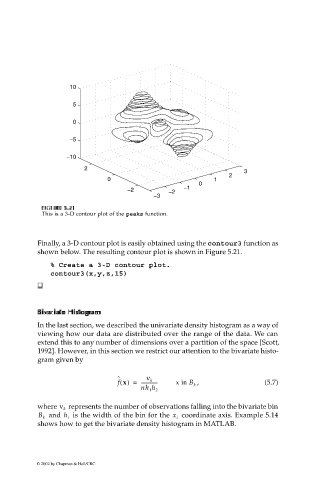
This is a 3-D contour plot of the peaks function.
Finally, a 3-D contour plot is easily obtained using the contour3 function as
shown below. The resulting contour plot is shown in Figure 5.21.

% Create a 3-D contour plot.
contour3(x,y,z,15)

HistoHisto
Biva
raamm
g
Biv
riat iate
ar
ee
BivBiv aarr iatiat eHistoHisto gr ggrr aamm
In the last section, we described the univariate density histogram as a way of
viewing how our data are distributed over the range of the data. We can
extend this to any number of dimensions over a partition of the space [Scott,
1992]. However, in this section we restrict our attention to the bivariate histo-
gram given by
ˆ ν k
f x() = -------------- x in B , (5.7)
k
nh 1 h 2
represents the number of observations falling into the bivariate bin
where ν k
coordinate axis. Example 5.14
B k and h i is the width of the bin for the x i
shows how to get the bivariate density histogram in MATLAB.

© 2002 by Chapman & Hall/CRC