Page 142 - Computational Statistics Handbook with MATLAB

Chapter 5: Exploratory Data Analysis 129

As we will see in the following example where we apply the modified Pois-
sonness plot to the word frequency data, the main effect of the modified plot
is to highlight those data points with small counts that do not behave con-
trary to the other observations. Thus, if a point that is plotted as a 1 in a mod-
ified Poissonness plot seems different from the rest of the data, then it should
be investigated.

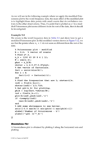
Example 5.8
We return to the word frequency data in Table 5.1 and show how to get a
modified Poissonness plot. In this modified version shown in Figure 5.12, we
see that the points where n k = 1 do not seem so different from the rest of the
data.
% Poissonness plot - modified
k = 0:6; % vector of counts
% Find n*_k.
n_k = [156 63 29 8 4 1 1];
N = sum(n_k);
phat = n_k/N;
nkstar = n_k-0.67-0.8*phat;
% Get vector of factorials.
fact = zeros(size(k));
for i = k
fact(i+1) = factorial(i);
end
% Find the frequencies that are 1; nkstar=1/e.
ind1 = find(n_k==1);
nkstar(ind1)= 1/2.718;
% Get phi(n_k) for plotting.
phik = log(fact.*nkstar/N);
ind = find(n_k~=1);
plot(k(ind),phik(ind),'o')
if ~isempty(ind1)
text(k(ind1),phik(ind1),'1')
end
% Add some whitespace to see better.
axis([-0.5 max(k)+1 min(phik)-1 max(phik)+1])
xlabel('Number of Occurrences - k')
ylabel('\phi (n^*_k)')

Plo
Plo
Binomialnes
Binomialnes s s s s Plo t Plo tt t
Binomialnes
Binomialnes
A binomialness plot is obtained by plotting k along the horizontal axis and
plotting
© 2002 by Chapman & Hall/CRC