Page 145 - Computational Statistics Handbook with MATLAB

132 Computational Statistics Handbook with MATLAB

−5
−5.5 1
−6
−6.5
−7
φ (n * ) k −7.5

−8 1
−8.5
−9
−9.5 1
−10

0 1 2 3 4 5 6 7 8 9 10
Number of Females − k

F FI IG URE G 5.1 RE 5.1 3 3
U
5.1
F F II GU RE RE 5.1 3 3
GU
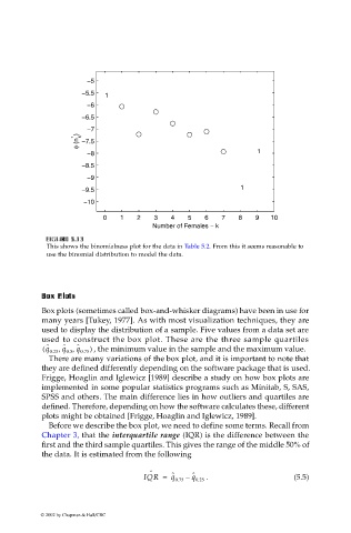
This shows the binomialness plot for the data in Table 5.2. From this it seems reasonable to
use the binomial distribution to model the data.

Bo xPlots Plots PlotsPlots
xx
x
Bo
BoBo
Box plots (sometimes called box-and-whisker diagrams) have been in use for
many years [Tukey, 1977]. As with most visualization techniques, they are
used to display the distribution of a sample. Five values from a data set are
used to construct the box plot. These are the three sample quartiles
,
ˆ
ˆ
( q 0.25 q 0.5 q 0.75 ) , the minimum value in the sample and the maximum value.
,
ˆ
There are many variations of the box plot, and it is important to note that
they are defined differently depending on the software package that is used.
Frigge, Hoaglin and Iglewicz [1989] describe a study on how box plots are
implemented in some popular statistics programs such as Minitab, S, SAS,
SPSS and others. The main difference lies in how outliers and quartiles are
defined. Therefore, depending on how the software calculates these, different
plots might be obtained [Frigge, Hoaglin and Iglewicz, 1989].
Before we describe the box plot, we need to define some terms. Recall from
Chapter 3, that the interquartile range (IQR) is the difference between the
first and the third sample quartiles. This gives the range of the middle 50% of
the data. It is estimated from the following
ˆ
IQR = ˆ q 0.75 – ˆ q 0.25 . (5.5)

© 2002 by Chapman & Hall/CRC