Page 166 - DSP Integrated Circuits

4.16 Design of Wave Digital Filters 151

can be uniquely mapped onto commensurate-length transmission line networks
using Richards' variable. However, some types of transmission line filter do not
have a lumped counterpart so they must be designed directly in the ^-domain.
Further, certain reference structures result in wave digital filter algorithms that
are not sequentially computable, because the wave-flow graph contains delay-free
loops (see Chapter 6).
One of the main obstacles is therefore to avoid these delay-free loops. There
are three major approaches used to avoid delay-free loops in wave digital filters:
1. By using certain types of reference filters that result directly in
sequentially computable algorithms. Such structures are
a. Cascaded transmission lines, so-called Richards' structures
b. Lattice filters with the branches realized by using circulators
c. Certain types of circulator filters [10, 30]
2. By introducing transmission lines between cascaded two-ports [10]
3. By using so-called reflection-free ports [8,10]
Naturally, combinations of these methods can also be used.

4.16.1 Feldtkeller's Equation
The low-sensitivity property of doubly resistively terminated LC filters that wave
digital filters inherit can be explained by Feldtkeller's equation:

where H = Bs/Aj is the normal transfer function and H c = B\IAi is the complemen-
tary transfer function. The outputs b\(n) and b^ji) are indicated in Figure 4.39.
The normal output is the voltage across the load resistor R§ while the complemen-
tary output is the voltage across RI in the reference filter.
The power delivered by the source will be dissipated in the two resistors, since
the reactance network is lossless. Thus, Feldtkeller's equation is a power relation-
ship. The complementary transfer function is often called the reflection function.
The maximum value of the magnitude of the reflection function in the passband is
called the reflection coefficient and is denoted by p. Hence, we have

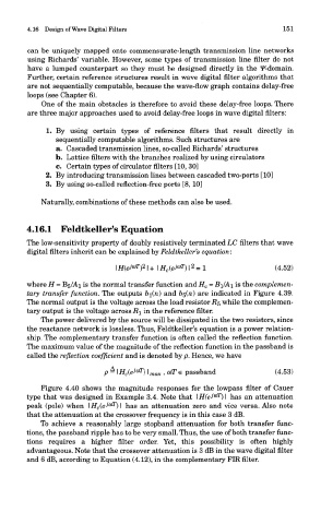
Figure 4.40 shows the magnitude responses for the lowpass filter of Cauer
(cir
type that was designed in Example 3.4. Note that \H(eJ )\ has an attenuation
)T
peak (pole) when \H c(eJ° )\ has an attenuation zero and vice versa. Also note
that the attenuation at the crossover frequency is in this case 3 dB.
To achieve a reasonably large stopband attenuation for both transfer func-
tions, the passband ripple has to be very small. Thus, the use of both transfer func-
tions requires a higher filter order. Yet, this possibility is often highly
advantageous. Note that the crossover attenuation is 3 dB in the wave digital filter
and 6 dB, according to Equation (4.12), in the complementary FIR filter.