Page 309 - DSP Integrated Circuits

294 Chapter 7 DSP System Design

7.5.1 Single Interval Scheduling Formulation

The starting point for scheduling is
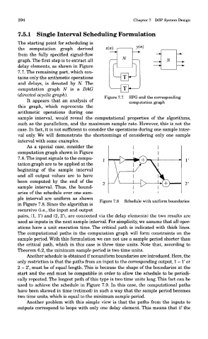
the computation graph derived
from the fully specified signal-flow
graph. The first step is to extract all
delay elements, as shown in Figure
7.7. The remaining part, which con-
tains only the arithmetic operations
and delays, is denoted by N. The
computation graph N is a DAG
(directed acyclic graph}.
Figure 7.7 SFG and the corresponding
It appears that an analysis of computation graph
this graph, which represents the
arithmetic operations during one
sample interval, would reveal the computational properties of the algorithms,
such as the parallelism, and the maximum sample rate. However, this is not the
case. In fact, it is not sufficient to consider the operations during one sample inter-
val only. We will demonstrate the shortcomings of considering only one sample
interval with some examples.
As a special case, consider the
computation graph shown in Figure
7.8. The input signals to the compu-
tation graph are to be applied at the
beginning of the sample interval
and all output values are to have
been computed by the end of the
sample interval. Thus, the bound-
aries of the schedule over one sam-
ple interval are uniform as shown
Figure 7.8 Schedule with uniform boundaries
in Figure 7.8. Since the algorithm is
recursive (i.e., the input and output
pairs, (1, 1') and (2, 2'), are connected via the delay elements) the two results are
used as inputs in the next sample interval. For simplicity, we assume that all oper-
ations have a unit execution time. The critical path is indicated with thick lines.
The computational paths in the computation graph will form constraints on the
sample period. With this formulation we can not use a sample period shorter than
the critical path, which in this case is three time units. Note that, according to
Theorem 6.2, the minimum sample period is two time units.
Another schedule is obtained if nonuniform boundaries are introduced. Here, the
only restriction is that the paths from an input to the corresponding output, 1 - 1' or
2 - 2', must be of equal length. This is because the shape of the boundaries at the
start and the end must be compatible in order to allow the schedule to be periodi-
cally repeated. The longest path of this type is two time units long. This fact can be
used to achieve the schedule in Figure 7.9. In this case, the computational paths
have been skewed in time (retimed) in such a way that the sample period becomes
two time units, which is equal to the minimum sample period.
Another problem with this simple view is that the paths from the inputs to
outputs correspond to loops with only one delay element. This means that if the