Page 312 - DSP Integrated Circuits

7.5 Scheduling Formulations 297

7.5.2 Block Scheduling Formulation

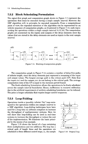
The signal-flow graph and computation graph shown in Figure 7.7 represent the
operations that must be executed during a single sample interval. However, the
DSP algorithm will, in principle, be executed repeatedly. From a computational
point of view, the repeated execution of the algorithm can be represented by an
infinite sequence of computation graphs, as illustrated in Figure 7.14, each repre-
senting the operations within a single sample interval [4, 8, 24]. The computation
graphs are connected via the inputs and outputs of the delay elements since the
values that are stored in the delay elements are used as inputs to the next sample
interval.

Figure 7.14 Blocking of computation graphs

The computation graph in Figure 7.14 contains a number of delay-free paths
of infinite length, since the delay elements just represent a renaming of the input
and output values. The longest average path is the critical path (CP). Note that
the input x(ri) and the output y(n) do not belong to the critical path. The average
computation time of the CP is equal to the iteration period bound.
The block scheduling formulation allows the operations to be freely scheduled
across the sample interval boundaries. Hence, inefficiency in resource utilization
due to the artificial requirement of uniform scheduling boundaries can be reduced.
The price is longer schedules that require longer control sequences.

7.5.3 Loop-Folding
Operations inside a (possibly infinite) for -loop corre-
spond to the operations within one sample interval in
a DSP algorithm. Loop-folding techniques have been
used for a long time in software compilers to increase
the throughput of multiprocessor systems. Here we
will show that loop-folding can be used in real-time
systems to increase the throughput or reduce the cost
of the implementation. We illustrate the basic princi-
ple by the means of an example.
Figure 7.15 shows the kernel of a loop containing
three multiplications and two additions. The loop has a
critical path of length three and the operations are
scheduled in three different control steps, i.e., the sample Figure 7.15 Original loop