Page 311 - Design and Operation of Heat Exchangers and their Networks

Optimal design of heat exchanger networks 297

Example H5C5—cont’d

588.93
433 366
H1
(8.79)
341.3 762
522 (8.690022) 411
H2
(10.55)
544 (4.985504) 422
H3
(12.56)
821.17
1556.8
500 339
H4
(14.77)
1300.3
472 339
H5
(17.73)
1057.79
450 355
(17.28) C1
478 366
C2
(13.9)
494 311
C3
(8.44)
955.59
433 333 C4
(7.62)
495 389 C5
(6.08)
(5.305256)
67.75
576.73
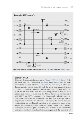
Fig. 6.28 Optimal solution for Example H5C5, TAC¼43,314$/yr (Toffolo, 2009).
Example H6C4
This example was originally proposed by Ahmad (1985, p.146, Table 5.3).It
has been used as a benchmark by many other researchers. In most
publications, the data listed in Table 6.29 have been used, in which the
thermal capacity rate of stream C3 and the target temperature of stream
H5 have been changed from the original values of 195kW/K and 85°C
to 180kW/K and 86°C, and the outlet temperatures of hot and cold
utilities that were not mentioned by Ahmad have been supplemented
with 198°C and 20°C, respectively. In this example, all units have the
same overall heat transfer coefficient, and the heat exchanger cost is
proportional to the area for all units. That means, the optimal network
configuration can be obtained according to the composite curves at the
optimal minimum temperature difference, which consists of a lot of heat
exchangers and stream splits. Therefore, this example is not suitable for
testing new synthesis procedures being developed, and the restriction of

Continued