Page 313 - Design and Operation of Heat Exchangers and their Networks

Optimal design of heat exchanger networks 299

Example H6C4—cont’d

1717
3457.823 1077.618
H1 85 45
(156.3) 1551.551
258.719 1190.599 999
H2 120 40
(50)
382.132 564
770 384.361 50.490 35
125
H3 (23.9)
H4 56 46
(1250)
3679 2321 12500
90 86
H5 (1500) 574.632
701.430 4342.490 1301 580.660
225 75
H6
(50)
55 40
(466.7) C1
65 55 C2
(600)
12956
165 65 C3
(180)
7430
170 10 C4
(81.3)
(A)
2315
H1 85 45
(156.3)
1143 2857
H2 120 40
(50)
2151
125
H3 (23.9) 35
12500
H4 56 46
(1250)
2936 3064 86
90
H5 (1500)
5579.207 1921
H6 225 75
(50)
55 40 C1
(466.7)
3936.783
65 55
(600) C2
12421
165 (204.1828) 65 C3
(180)
170 10
(81.3) C4
(B) 8000 (30.81177)
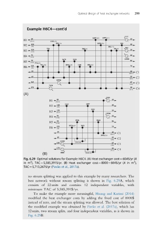
Fig. 6.29 Optimal solutions for Example H6C4. (A) Heat exchanger cost¼60A$/yr (A
2
2
in m ), TAC¼5,585,391$/yr. (B) Heat exchanger cost¼8000+60A$/yr (A in m ),
TAC¼5,713,267$/yr (Pavão et al., 2017a).
no stream splitting was applied to this example by many researchers. The
best network without stream splitting is shown in Fig. 6.29A, which
consists of 22units and contains 12 independent variables, with
minimum TAC of 5,585,391$/yr.
To make the example more meaningful, Huang and Karimi (2014)
modified the heat exchanger costs by adding the fixed cost of 8000$
instead of zero, and the stream splitting was allowed. The best solution of
the modified example was obtained by Pava ˜o et al. (2017a), which has
12units, two stream splits, and four independent variables, as is shown in
Fig. 6.29B.