Page 317 - Design and Operation of Heat Exchangers and their Networks

Optimal design of heat exchanger networks 303

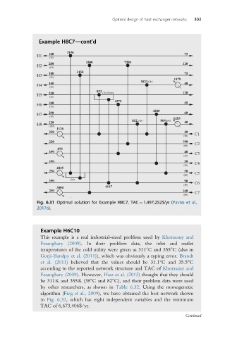
Example H8C7—cont’d

3150
180 75
H1
(30)
280 2400 7200 120
H2
(60)
180 3150 75
H3
(30)
1179
1821.014
140 40
H4
(30)
853
220 (10.29220) 120
H5
(50)
4375
180 55
H6
(35)
4200
200 60
H7
(30)
6283
852.769 864.645
120 40
H8
(100)
1126
230 40
(20) C1
220 100 C2
(60)
875
190 40
C3
(35)
190 50 C4
(30)
4835
250 50
(60) C5
190 (30) 90
C6
(50)
3000 4147
250 160
C7
(60)
Fig. 6.31 Optimal solution for Example H8C7, TAC¼1,497,252$/yr (Pavão et al.,
2017a).
Example H6C10
This example is a real industrial-sized problem used by Khorasany and
Fesanghary (2009). In their problem data, the inlet and outlet
temperatures of the cold utility were given as 311°C and 355°C (also in
Gorji-Bandpy et al. (2011)), which was obviously a typing error. Brandt
et al. (2011) believed that the values should be 31.1°C and 35.5°C
according to the reported network structure and TAC of Khorasany and
Fesanghary (2009). However, Huo et al. (2013) thought that they should
be 311K and 355K (38°C and 82°C), and their problem data were used
by other researchers, as shown in Table 6.32. Using the monogenetic
algorithm (Fieg et al., 2009), we have obtained the best network shown
in Fig. 6.32, which has eight independent variables and the minimum
TAC of 6,673,406$/yr.
Continued