Page 378 - Design and Operation of Heat Exchangers and their Networks

Dynamic analysis of heat exchangers and their networks 361

The final solution of temperature response in the Laplace domain is then
expressed as
1 0 0
0
Θ xðÞ ¼ V xðÞ V 2GV 00 G Θ (7.209)
e e
e
e
Substituting Eq. (7.209) into Eq. (7.201), we also obtain the temperature
responses at the exchanger outlets as
n h io
00 000 00 1 0 0
0
00
Θ ¼ G + G V V 2GV 00 G Θ (7.210)
e
e
e
e
e
e
The real-time solution can be obtained with the FFT algorithm,
Eq. (2.178).
Example 7.1 Dynamic responses of a 1–3 shell-and-tube
heat exchanger.
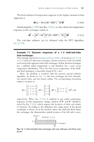
This example is given by Roetzel and Xuan (1992c). As shown in Fig. 7.4,it
is a 1–3 shell-and-tube heat exchanger, and the entrances of the two fluids
are located at the opposite ends of the exchanger. At first, the heat exchanger
has a uniform initial temperature t 0 and therefore has a zero excess
temperature distribution. Then, the inlet excess temperature of the shell-
side fluid undergoes a sinusoidal change θ 1 (τ)¼sinτ.
0
Here, the problem is resolved with the present general solution
algorithm. As shown in Fig. 7.4, the heat exchanger has four channels,
two stream inlets, and two stream outlets. The corresponding connecting
matrices are given as
2 3 2 3
00 00 01

6 10 00 7 6 00 7 000 1
00
000
0
G ¼ 6 7 , G ¼ 6 7 , G ¼ , G ¼ 0
4 01 00 5 4 00 5 001 0
00 00 10
respectively. When Eq. (7.210) is adopted to get outlet temperature
0
responses of inlet temperature change, matrices of V and V should be
00
solved by Eq. (7.206), which requires the locations of inlets and outlets
of channels. According to the definition that origin point of the spatial
coordinate is always set at the location where the shell-side fluid enters
the exchanger, the dimensionless spatial location of the left side is zero,
Stream 1
Channel 1, 2, 3, 4

Stream 2

Fig. 7.4 A shell-and-tube heat exchanger with one shell pass and three tube
passes.