Page 284 - Digital Analysis of Remotely Sensed Imagery

246 Cha pte r S i x

cosine

sine
0 π 2π 0 π 2π

(a) (b)

0 π 2π
(c)
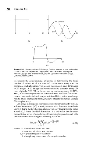
FIGURE 6.26 Decomposition of 1D image ƒ(x) into a series of sine and cosine
curves of various frequencies, magnitudes, and coeffi cients. (a) Original
function ƒ(x); (b) sine and cosine of ƒ(x); and (c) Fourier transform of ƒ(x).
(Source: Mather, 2004)

to expedite the computational efficiency in determining the huge
number of values for all the sine and cosine terms along with the
coefficient multiplications. The second extension is from 1D images
to 2D images. A 2D image can be considered to comprise many 1D
rows of pixels. A 2D FFT can be devised by combining many 1D FFTs.
Thus, the scale components are 2D waveforms, and each scale com-
ponent has an orientational component, in addition to the usual mag-
nitude. These coefficients form 2D arrays of real numbers or a single
2D complex array.
An image in the spatial domain is denoted mathematically as f(i, j),
a three-dimensional (3D) intensity surface with the rows (i) and col-
umns (j) being the two horizontal axes. The gray-level intensity value
at each (i, j) forms the third dimension. It is this value that is trans-
formed into a series of waveforms of increasing frequencies and with
different orientations using the following equation:
M−1 N−1 −2π ⎛ ⎜ ux + uy⎞ ⎟
Fu v) = ∑ ∑ ∑ f i j e ⎝ M N ⎠ (6.27)
,
(
)
(,
x=0 y=0
where M = number of pixels in a row
N = number of pixels in a column
u, v = spatial frequency variables
k = imaginary component of a complex number