Page 279 - Digital Analysis of Remotely Sensed Imagery

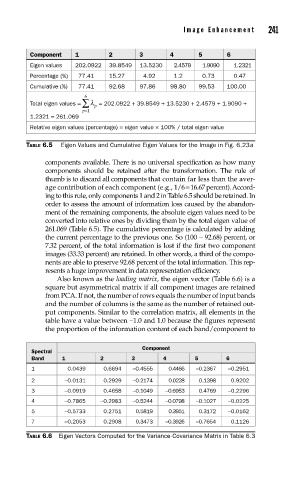
Image Enhancement 241

Component 1 2 3 4 5 6
Eigen values 202.0922 39.8549 13.5230 2.4579 1.9090 1.2321
Percentage (%) 77.41 15.27 4.92 1.2 0.73 0.47
Cumulative (%) 77.41 92.68 97.86 98.80 99.53 100.00
6
Total eigen values = ∑ λ = 202.0922 + 39.8549 + 13.5230 + 2.4579 + 1.9090 +
p=1 p
1.2321 = 261.069
Relative eigen values (percentage) = eigen value × 100% / total eigen value

TABLE 6.5 Eigen Values and Cumulative Eigen Values for the Image in Fig. 6.23a

components available. There is no universal specification as how many
components should be retained after the transformation. The rule of
thumb is to discard all components that contain far less than the aver-
age contribution of each component (e.g., 1/6 = 16.67 percent). Accord-
ing to this rule, only components 1 and 2 in Table 6.5 should be retained. In
order to assess the amount of information loss caused by the abandon-
ment of the remaining components, the absolute eigen values need to be
converted into relative ones by dividing them by the total eigen value of
261.069 (Table 6.5). The cumulative percentage is calculated by adding
the current percentage to the previous one. So (100 − 92.68) percent, or
7.32 percent, of the total information is lost if the first two component
images (33.33 percent) are retained. In other words, a third of the compo-
nents are able to preserve 92.68 percent of the total information. This rep-
resents a huge improvement in data representation efficiency.
Also known as the loading matrix, the eigen vector (Table 6.6) is a
square but asymmetrical matrix if all component images are retained
from PCA. If not, the number of rows equals the number of input bands
and the number of columns is the same as the number of retained out-
put components. Similar to the correlation matrix, all elements in the
table have a value between −1.0 and 1.0 because the figures represent
the proportion of the information content of each band/component to

Component
Spectral
Band 1 2 3 4 5 6
1 0.0439 0.6694 −0.4555 0.4466 −0.2367 −0.2951
2 −0.0131 0.2929 −0.2174 0.0228 0.1398 0.9202
3 −0.0919 0.4658 −0.1049 −0.6953 0.4769 −0.2296
4 −0.7865 −0.2983 −0.5244 −0.0798 −0.1027 −0.0225
5 −0.5733 0.2751 0.5819 0.3951 0.3172 −0.0162
7 −0.2053 0.2908 0.3473 −0.3926 −0.7654 0.1126
TABLE 6.6 Eigen Vectors Computed for the Variance-Covariance Matrix in Table 6.3