Page 281 - Digital Analysis of Remotely Sensed Imagery

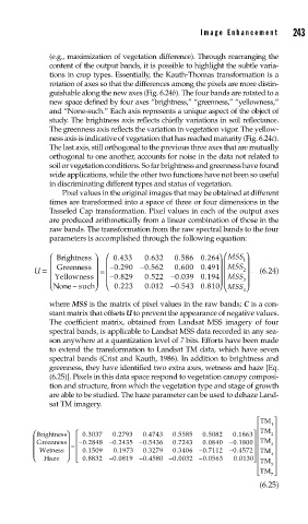
Image Enhancement 243

(e.g., maximization of vegetation difference). Through rearranging the
content of the output bands, it is possible to highlight the subtle varia-
tions in crop types. Essentially, the Kauth-Thomas transformation is a
rotation of axes so that the differences among the pixels are more distin-
guishable along the new axes (Fig. 6.24b). The four bands are rotated to a
new space defined by four axes “brightness,” “greenness,” “yellowness,”
and “None-such.” Each axis represents a unique aspect of the object of
study. The brightness axis reflects chiefly variations in soil reflectance.
The greenness axis reflects the variation in vegetation vigor. The yellow-
ness axis is indicative of vegetation that has reached maturity (Fig. 6.24c).
The last axis, still orthogonal to the previous three axes that are mutually
orthogonal to one another, accounts for noise in the data not related to
soil or vegetation conditions. So far brightness and greenness have found
wide applications, while the other two functions have not been so useful
in discriminating different types and status of vegetation.
Pixel values in the original images that may be obtained at different
times are transformed into a space of three or four dimensions in the
Tasseled Cap transformation. Pixel values in each of the output axes
are produced arithmetically from a linear combination of those in the
raw bands. The transformation from the raw spectral bands to the four
parameters is accomplished through the following equation:
⎛ Brightness ⎞ ⎞ ⎛ 0 433 0 632 0 586 0 264⎞ ⎛MSS 1 ⎞
.
.
.
.
⎜ Greenness ⎟ ⎜ 0 491 ⎟ ⎜ ⎟
.
.
.
U = ⎜ ⎟ = ⎜ −0 290 −0 562 0 6000 . ⎟ ⎜ MSS 2 ⎟ ⎟ + (6.24)
.
.
.
.
⎜ Yellowness ⎟ ⎜ − 0 829 0 522 − 0 039 0 194 ⎟ ⎜ MSS 3⎟
⎜
⎝ None such⎠ ⎝ 0 223 0 012 − 0 5 . 443 0 810⎠ ⎝ MSS 4 ⎠ ⎟
−
.
.
.
where MSS is the matrix of pixel values in the raw bands; C is a con-
stant matrix that offsets U to prevent the appearance of negative values.
The coefficient matrix, obtained from Landsat MSS imagery of four
spectral bands, is applicable to Landsat MSS data recorded in any sea-
son anywhere at a quantization level of 7 bits. Efforts have been made
to extend the transformation to Landsat TM data, which have seven
spectral bands (Crist and Kauth, 1986). In addition to brightness and
greenness, they have identified two extra axes, wetness and haze [Eq.
(6.25)]. Pixels in this data space respond to vegetation canopy composi-
tion and structure, from which the vegetation type and stage of growth
are able to be studied. The haze parameter can be used to dehaze Land-
sat TM imagery.
⎡ TM ⎤
⎢ 1 ⎥
⎛ Brightness⎞ ⎡ 0.33037 0 2793 0 4743 0 5585 0 5082 0 1863⎤ ⎢ TM 2 ⎥
.
.
.
.
.
⎜ Greenness⎟ ⎢ − 0 2848 −0 2435 − 0 5436 0 7243 0 0840 − 0 1800⎥ TTM 3⎥
⎢
.
.
.
.
.
.
0
=
⎜ Wetness ⎟ ⎢ 0 1509 0 19773 0 3279 0 3406 − 0 7112 − 0 4572 ⎥ ⎢ TM ⎥
.
.
.
.
.
.
⎜ ⎝ Haze ⎠ ⎟ ⎢ − −0 4580 − 0 0032 − 0 0130 ⎢ 4 ⎥
⎥
⎣
.
0 8832
.
.
0 0819
0
0 0563
.
.
.
⎦ TM
⎢ 5⎥
⎢ ⎣ TM ⎥
7⎦
(6.25)