Page 233 - Dynamic Loading and Design of Structures

Page 205

●generate time series for the wave kinematics at discrete points along the structure by FFT;
●calculate corresponding loads by the Morison equation, and equivalent nodal forces;
●perform step by step integration of dynamic equations of motion, using methods mentioned
in Section 5.4.2.
Finally, having obtained the response histories, and properly eliminated spurious start
transients, statistical inference and estimation of relevant response quantities (variances,
extremes) can be carried out. Filtering of the response may be considered especially in cases
where the wave loading causes a combination of steady-state and transient response, and the
transient part is deterministic when it has been initiated.
Limited sampling size introduces uncertainties, which may be quite significant for extreme
values. It is particularly necessary to extrapolate from a limited sample size (say, half an hour)
to extreme values in a short-term period of, say, 3–6 hours. Theoretical results are available
for the distribution of individual response maxima of single cylinders with static response to
non-linear loads associated with drag forces and surface elevation (e.g. Brouwers and
Verbeek, 1983). For multi-DOF systems with dynamic behaviour only empirical studies of
best fit can be made. A three-parameter Weibull distribution or a Weibull tail method (see e.g.
Farnes, 1990) or Hermite models (see e.g. Winterstein, 1988) are frequently applied for this
purpose.

5.4.4 Frequency domain analysis
FDAs outlined in the following are based on linearization of the system model. Like the
surface elevation variation, load effect processes are then implicitly assumed to be Gaussian.
The distribution of individual peaks or stress ranges, and expected maxima in a given short
term period may then be achieved for single response quantities according to well known
theory, see Chapter 10. Parameters, such as variance and spectral width, can be obtained from
the response spectrum Sr(ω) for the response r in eqn (5.45).
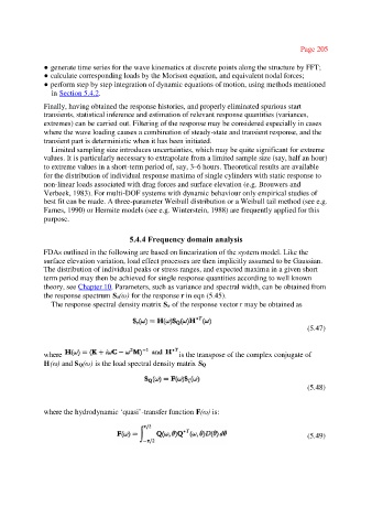
The response spectral density matrix Sr of the response vector r may be obtained as

(5.47)

where is the transpose of the complex conjugate of
)
H(ω and SQ(ω) is the load spectral density matrix S Q

(5.48)

where the hydrodynamic ‘quasi’-transfer function F(ω is:
)

(5.49)