Page 276 - Dynamics of Mechanical Systems

0593_C08_fm Page 257 Monday, May 6, 2002 2:45 PM

Principles of Dynamics: Newton’s Laws and d’Alembert’s Principle 257

2

θ
m /2 O y
O
x
θ
¨

m /2 2
(1/3)m θ ¨
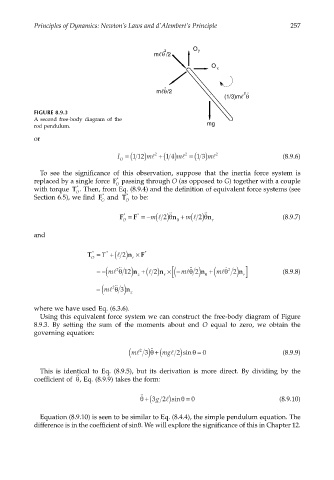
FIGURE 8.9.3
A second free-body diagram of the
rod pendulum. mg
or

I = (112 m ) l 2 +(1 m ) 4 l 2 = (1 m ) 3 l 2 (8.9.6)
O
To see the significance of this observation, suppose that the inertia force system is
replaced by a single force F O * passing through O (as opposed to G) together with a couple
with torque T * . Then, from Eq. (8.9.4) and the definition of equivalent force systems (see
O
Section 6.5), we find F * and T * to be:
O O
F = F = − m(l ˙˙ n ) 2 θ + m(l ˙˙ n ) 2 θ (8.9.7)
*
*
O θ r
and

T = T +(l n ) 2 × F *
*
*
O r
=−( ml θ n ) n ) [ mlθ + m ( lθ ˙ 2 r]
r (
˙˙
×−
˙˙
2
12
z +(l 2 n ) 2 θ n ) 2 (8.9.8)
˙˙
= m ( l θ n ) 3
2
z
where we have used Eq. (6.3.6).
Using this equivalent force system we can construct the free-body diagram of Figure
8.9.3. By setting the sum of the moments about end O equal to zero, we obtain the
governing equation:
( ml 3) +( mgl 2)sinθ = 0 (8.9.9)
θ
˙˙
2
This is identical to Eq. (8.9.5), but its derivation is more direct. By dividing by the
θ
˙˙
coefficient of , Eq. (8.9.9) takes the form:
˙˙ θ +(3g 2l ) sinθ = 0 (8.9.10)

Equation (8.9.10) is seen to be similar to Eq. (8.4.4), the simple pendulum equation. The
difference is in the coefficient of sinθ. We will explore the significance of this in Chapter 12.