Page 281 - Dynamics of Mechanical Systems

0593_C08_fm Page 262 Monday, May 6, 2002 2:45 PM

262 Dynamics of Mechanical Systems

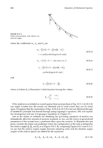
FIGURE 8.11.3
Triple-rod pendulum with relative ori-
entation angles.
where the coefficients m , n , and k are:
rj
rj
rj
rj [
]
−
m = ( ) + N q cos θ r ( − θ j)
2
1
(8.11.5)
j
r
r ≠ and isthelargestof and j
q
−
m = ( ) − N r ( no sum on r) (8.11.6)
3
1
rr
rj [
]
−
n = ( ) + N q sin θ r ( − θ j) ,
1
2
(8.11.7)
r
qisthelargestof and j
and
rj [
k = ( ) + N − δ rj ] (8.11.8)
12
j
where as before δ is Kronecker’s delta function having the values:
rj
0 r ≠ j
δ =  (8.11.9)
rj r =
 1 j
If the analysis is as detailed as would appear from an inspection of Eqs. (8.11.1) to (8.11.8)
one might wonder how the results are obtained and to what extent they can be relied
upon. It happens that the expressions of Eqs. (8.11.1) to (8.11.8) were not obtained through
d’Alembert’s principle but instead through using Lagrange’s equations. (We will explore
the development and use of Lagrange’s equations in Chapter 11.)
Just as the choice of methods for obtaining the governing equations of motion can
dramatically affect the amount of analysis required, so, too, can the choice of geometrical
parameters of the system have a profound effect upon the analysis. To illustrate this last
point, consider the triple-rod pendulum where the configuration of the rods is defined by
the relative angles β , β , and β as in Figure 8.11.3. By comparing Figures 8.11.1 and 8.11.3,
2
1
3
we see that the relative angles (angles between adjoining rods) and the absolute angles
(angles of the rods in space) are related by the equations:
θ = β , θ = β + β , θ = β + β + β (8.11.10)
1 1 2 1 2 3 1 2 3