Page 52 - Electric Drives and Electromechanical Systems

Chapter 2 Analysing a drive system 45

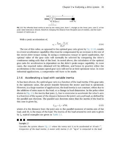
FIG. 2.5 The effective load inertia as seen by the rotary joint, Joint 1, changes as the linear joint, Joint 2, of the
polar robot extends or retracts, therefore changing the distance from the joints axis of rotation, and the load’s
moment of inertia axis, d.

With a peak acceleration of,
T peak T L =n
a L ¼ (2.14)
2I m n
The use of this value, as opposed to the optimal gear ratio given by Eq. (2.10), results
in a lower acceleration capability; this must be compensated by an increase in the size of
the motor-drive torque rating. In sizing a continuous torque or speed application, the
optimal value of the gear ratio will normally be selected by comparing the drive’s
continuous rating with that of the load. As noted above, the calculation of the optimal
gear ratio for acceleration is dependent on the drive’s peak-torque capability. In most
cases, the required ratios obtained will be different, and hence in practice either the
acceleration or the constant-speed gear ratio will not be at their optimum value. In most
industrial applications, a compromise will have to be made.

2.1.6 Accelerating a load with variable inertia

As has been shown, the optimal gear ratio is a function of the load inertia: if the gear ratio
is the optimum value, the power transfer between the motor and load is optimised.
However, in a large number of applications, the load inertia is not constant, either due to
the addition of extra mass to the load, or a change in load dimension. In the polar robot
shown in Fig. 2.5; the inertia that joint, J 1 , has to overcome to accelerate the robot’s arm
is a function of the square of the distance between the joint’s axis and load, as defined by
the parallel axis theorem. The parallel axis theorem states that the inertia of the load in
this case is given by,
2 (2.15)
I Load ¼ I a þ d M L
where d is the distance from the joint axis to the parallel moment of inertia axis of the
load, and M L is the mass of the load. The inertia of the load around its own axis is given
by I a , typical examples are given in Table 2.1.
nnn
Example 2.1
2
Consider the system shown Fig. 2.5 where the rotary axis is to be accelerated at 10 rad s ,
2
irrespective of the load inertia. A motor with inertia 2 10 3 kg m is connected to the load