Page 431 - Electrical Properties of Materials

Effective permeability 413

where Q is the quality factor, defined as

ω 0 L
Q = . (15.21)
R
For the lossless case, with a little algebra, eqn (15.20) reduces to

2
2
(1 – F)(ω – ω )
F
μ r = 2 , (15.22)
2
(ω – ω )
0
where
μ 0 NS 2 ω 0
F = and ω F = . (15.23)
L (1 – F) 1/2
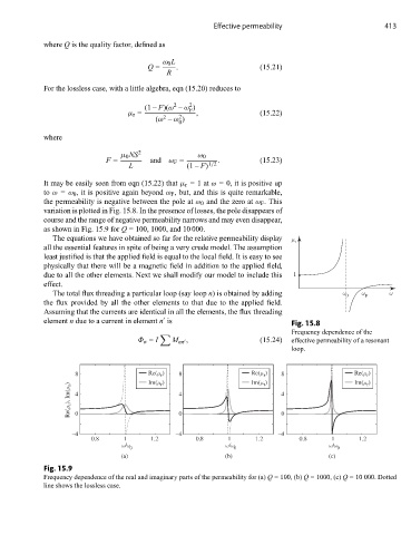
It may be easily seen from eqn (15.22) that μ r =1 at ω = 0, it is positive up
to ω = ω 0 , it is positive again beyond ω F , but, and this is quite remarkable,
the permeability is negative between the pole at ω 0 and the zero at ω F .This
variation is plotted in Fig. 15.8. In the presence of losses, the pole disappears of
course and the range of negative permeability narrows and may even disappear,
as shown in Fig. 15.9 for Q = 100, 1000, and 10 000.
The equations we have obtained so far for the relative permeability display μ r
all the essential features in spite of being a very crude model. The assumption
least justified is that the applied field is equal to the local field. It is easy to see
physically that there will be a magnetic field in addition to the applied field,
due to all the other elements. Next we shall modify our model to include this 1
effect.
The total flux threading a particular loop (say loop n) is obtained by adding ω 0 ω F ω
the flux provided by all the other elements to that due to the applied field.
Assuming that the currents are identical in all the elements, the flux threading
element n due to a current in element n is Fig. 15.8

Frequency dependence of the

Φ n = I M nn , (15.24) effective permeability of a resonant

loop.
8 Re(μ ) r 8 Re(μ ) r 8 Re(μ )
r
Im(μ ) r Im(μ ) r Im(μ )
r
Re(μ r ), Im(μ r ) 4 0 4 0 4 0

–4 –4 –4
0.8 1 1.2 0.8 1 1.2 0.8 1 1.2
ω/ω ω/ω ω/ω
0 0 0
(a) (b) (c)
Fig. 15.9
Frequency dependence of the real and imaginary parts of the permeability for (a) Q = 100, (b) Q = 1000, (c) Q = 10 000. Dotted
line shows the lossless case.