Page 295 - Elements of Distribution Theory

P1: JZP
052184472Xc09 CUNY148/Severini June 2, 2005 12:8

9.6 Uniform Asymptotic Approximations 281

E[log (1 + y 2 ); α]

α
2
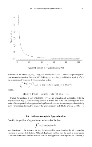
Figure 9.2. E[log(1 + Y ); α]in Example 9.11.

Note that, in the interval [1, ∞), − log(y)is maximized at y = 1; hence, a Laplace approxi-
2
mation must be based on Theorem 9.15. Taking g(y) =− log(y) and h(y) = log(1 + y )/y,
the conditions of Theorem 9.15 are satisfied so that
2
log(1 + y ) 1 −1
∞
exp{−α log(y)} dy = log(2) [1 + O(α )]
y α
1
so that
2
−1
E[log(1 + Y ); α] = log(2)[1 + O(α )] as α →∞.
2
Figure 9.2 contains a plot of E[log(1 + Y ); α]asa function of α, together with the
approximation log(2), which is displayed as a dotted line. Note that, although the exact
value of the expected value approaches log(2) as α increases, the convergence is relatively
slow. For instance, the relative error of the approximation is still 1.4% when α = 100.

9.6 Uniform Asymptotic Approximations

Consider the problem of approximating an integral of the form
∞

h(y)exp(ng(y)) dy,
z
as a function of z; for instance, we may be interested in approximating the tail probability
function of a given distribution. Although Laplace’s method may be used, in many cases,
it has the undesirable feature that the form of the approximation depends on whether ˆ y,