Page 572 - Engineering Digital Design

542 CHAPTER 11 / SYNCHRONOUS FSM DESIGN CONSIDERATIONS

functions:

D A = CSf + BCST + ACS + AT
D B = CST + BT
(11.11)
P = ACST
Q = ACS + BCST + ABC

These results represent a total gate/input tally of 14/40, excluding possible inverters.
Eqs. (11.11) will be compared with the results generated by using the array algebraic
approach to design discussed next in Section 11.11.

11.11 ARRAY ALGEBRAIC APPROACH TO LOGIC DESIGN

Results similar to those of Eqs. (11.11) can be obtained by using what is called the array
algebraic approach to state machine design. This approach is applicable to any FSM for
which each state-to-state transition ends in a holding condition, and each state obeys the
sum rule. Thus, the FSM in Fig. 11.36 would not be suitable for this method since there are
states without holding conditions.
The array algebraic approach can be used for the computer automated design (CAD) of
either synchronous or asynchronous FSMs, and without the need to use either state diagrams
or K-maps. Furthermore, the array algebra that is used bears a close resemblance to matrix
algebra, but there are some important differences. To properly launch this subject and to
minimize the difficulty index, the various matrix arrays and equations will be given using
the FSM in Fig. 11.43 as an example. In this way, the reader can follow the operations with
little difficulty.
Given the state code assignments that are generated by using the next-state table in
Fig. 11.43a,

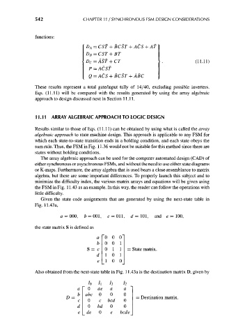
a =000, fc = 001, c = 011, d = 101, and e = 100,

the state matrix S is defined as
'0 0 0"
b 0 0 1
S= c 0 1 1 = State matrix.
d 1 0 1
e 1 0 0

Also obtained from the next-state table in Fig. 11.43a is the destination matrix D, given by

/o /i h h
a 0 ae a a
b abc 0 0 0
D = = Destination matrix.
c 0 c bed 0
d 0 bd 0 0
e de 0 e bcde