Page 571 - Engineering Digital Design

Sanity
1
\ST '° ' '3 >2
ABC\ 00 01 11 10
®
a b (a) (a) ab
b (W d c e ;bd,i be, cd, ce
V_x \

c b GD )© e be, ce, be
ST
d e ®' c e ;de,| cd, ce
\
_^ \
^^^
^~N
e (£) a (*) (e) ;ae j
I 1
T Rule 2
J abc ae bed bcde ^-^-—^ ^v^- PiT ifST
Rule 1 < CUT if S
1 Jdel bd
(a) (b)
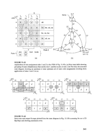
FIGURE 11.43
Application of state assignment rules 1 and 2 to the FSM of Fig. 11.42a. (a) Next state table showing
grouping of states (shaded areas) that satisfy rule 1, and the results of rule 2. (b) The fully documented
state diagram showing an optimum or near optimum set of state code assignments resulting from
application of rules 1 and 2 in (a).

JBC \BC \BC
00 01 11 10 A \ °° 01 11 10 AX °° 01 11 10
S®T ST ST ST S+T S-t-T 4>

+f ST 0 T
* *

,BC \BC
\ 00 01 11 10 A \ 00 01 11 10

ST
Xu
FIGURE 11.44
Next-state and output K-maps plotted from the state diagram in Fig. 11.43b assuming the use of D
flip-flops and showing minimum cover.

541