Page 758 - Engineering Digital Design

724 CHAPTER 14/ASYNCHRONOUS STATE MACHINE DESIGN AND ANALYSIS

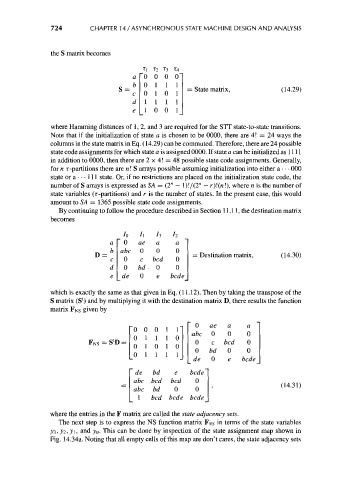
the S matrix becomes

TI ^2 ^3 T 4
a 0 0 0 0"
b 0 1 1 1
S = = State matrix, (14.29)
c 0 1 0 1
d 1 1 1 1
e 1 0 0 1

where Hamming distances of 1, 2, and 3 are required for the STT state-to-state transitions.
Note that if the initialization of state a is chosen to be 0000, there are 4! = 24 ways the
columns in the state matrix in Eq. (14.29) can be commuted. Therefore, there are 24 possible
state code assignments for which state a is assigned 0000. If state a can be initialized as 1111
in addition to 0000, then there are 2 x 4! = 48 possible state code assignments. Generally,
for n T-partitions there are n! S arrays possible assuming initialization into either a • • • 000
state or a • • • 111 state. Or, if no restrictions are placed on the initialization state code, the
n
number of S arrays is expressed as SA = (2 — l)!/(2" — r}\(n!), where n is the number of
state variables (T-partitions) and r is the number of states. In the present case, this would
amount to SA = 1365 possible state code assignments.
By continuing to follow the procedure described in Section 11.11, the destination matrix
becomes

/O /I /3 /2
0 ae a a
abc 0 0 0
= Destination matrix, (14.30)
0 c bed 0
d 0 W • 0 0
e de 0 e bcde

which is exactly the same as that given in Eq. (11.12). Then by taking the transpose of the
1
S matrix (S ) and by multiplying it with the destination matrix D, there results the function
matrix FNS given by

"0 0 0 i r " 0 ae a a
0 1 1 1 0 abc 0 0 0
F NS =S'D = 0 c bed 0
0 1 0 1 0 0 0 0
0 1 1 1 1 bd
de 0 e bcde
de bd e bcde
abc bed bed 0
(14.31)
abc bd 0 0
1 bed bcde bcde

where the entries in the F matrix are called the state adjacency sets.
The next step is to express the NS function matrix FJVS in terms of the state variables
J3, j2, vj, and y 0. This can be done by inspection of the state assignment map shown in
Fig. 14.34a. Noting that all empty cells of this map are don't cares, the state adjacency sets