Page 762 - Engineering Digital Design

728 CHAPTER 14 /ASYNCHRONOUS STATE MACHINE DESIGN AND ANALYSIS

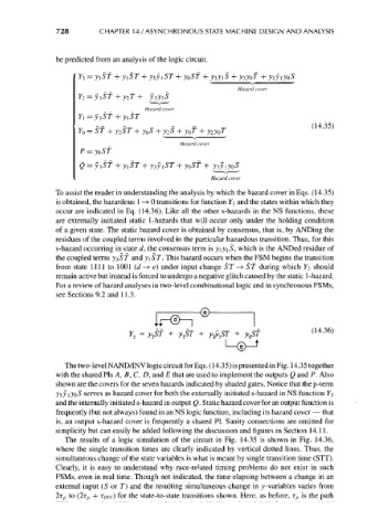
be predicted from an analysis of the logic circuit.
y\ST + y3y\ST + y 0ST +

Hazard cover

_ _ _ Hazard cover
Y }=y 3Sf+ yiST
YQ = ST + y 2ST + y 0S + y 2S
Hazard cover
P =

Hazard cover
To assist the reader in understanding the analysis by which the hazard cover in Eqs. (14.35)
is obtained, the hazardous 1 — > 0 transitions for function Y 3 and the states within which they
occur are indicated in Eq. (14.36). Like all the other s-hazards in the NS functions, these
are externally initiated static 1 -hazards that will occur only under the holding condition
of a given state. The static hazard cover is obtained by consensus, that is, by ANDing the
residues of the coupled terms involved in the particular hazardous transition. Thus, for this
s-hazard occurring in state d, the consensus term is y 3y\ 5, which is the ANDed residue of
the coupled terms y 3ST and y\ ST. This hazard occurs when the FSM begins the transition
from state 1111 to 1001 (d—^e~) under input change ST — »> ST during which Y 3 should
remain active but instead is forced to undergo a negative glitch caused by the static 1 -hazard.
For a review of hazard analyses in two-level combinational logic and in synchronous FSMs,
see Sections 9.2 and 1 1.3.

(14.36)
y tST

The two-level NAND/INV logic circuit for Eqs. (14.35) is presented in Fig. 14.35 together
with the shared Pis A, B, C, D, and E that are used to implement the outputs Q and P. Also
shown are the covers for the seven hazards indicated by shaded gates. Notice that the p-term
yiy \yoS serves as hazard cover for both the externally initiated s-hazard in NS function Y 3
and the internally initiated s-hazard in output Q. Static hazard cover for an output function is
frequently (but not always) found in an NS logic function, including its hazard cover — that
is, an output s-hazard cover is frequently a shared PI. Sanity connections are omitted for
simplicity but can easily be added following the discussion and figures in Section 14.1 1.
The results of a logic simulation of the circuit in Fig. 14.35 is shown in Fig. 14.36,
where the single transition times are clearly indicated by vertical dotted lines. Thus, the
simultaneous change of the state variables is what is meant by single transition time (STT).
Clearly, it is easy to understand why race-related timing problems do not exist in such
FSMs, even in real time. Though not indicated, the time elapsing between a change in an
external input (S or T) and the resulting simultaneous change in y- variables varies from
2r p to (2r p + TMV) for the state-to-state transitions shown. Here, as before, r p is the path