Page 552 - Engineering Electromagnetics, 8th Edition

534 ENGINEERING ELECTROMAGNETICS

S
y
r
d f
P
r 1

x
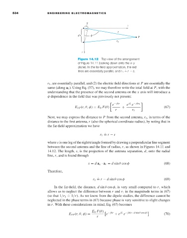
Figure 14.12 Top view of the arrangement
of Figure 14.11 (looking down onto the x-y
plane). In the far-field approximation, the red
.
lines are essentially parallel, and r 1 = r − s.

r 1 , are essentially parallel, and (2) the electric field directions at P are essentially the
same (along a θ ). Using Eq. (57), we may therefore write the total field at P, with the
understanding that the presence of the second antenna on the x axis will introduce a
φ dependence in the field that was previously not present:

e e e − jkr 1
− jkr jξ
E θ P (r,θ,φ) = E 0 F(θ) + (67)
r r 1
Next, we may express the distance to P from the second antenna, r 1 ,in terms of the
distance to the first antenna, r (also the spherical coordinate radius), by noting that in
the far-field approximation we have
.
r 1 = r − s

where s is one leg of the right triangle formed by drawing a perpendicular line segment
between the second antenna and the line of radius, r,as shown in Figures 14.11 and
14.12. The length, s,is the projection of the antenna separation, d, onto the radial
line, r, and is found through

s = d a x · a r = d sin θ cos φ (68)

Therefore,
.
r 1 = r − d sin θ cos φ (69)
In the far-field, the distance, d sin θ cos φ,isvery small compared to r, which
allows us to neglect the difference between r and r 1 in the magnitude terms in (67)
.
(so that 1/r 1 = 1/r). As we know from the dipole studies, the difference cannot be
neglected in the phase terms in (67) because phase is very sensitive to slight changes
in r.With these considerations in mind, Eq. (67) becomes

E 0 F(θ) − jkr jξ − jk(r−d sin θ cos φ)
E θ P (r,θ,φ) = e + e e (70)
r