Page 242 - Essentials of physical chemistry

204 Essentials of Physical Chemistry

1.0

Curve 1
0.8

0.6
Absorbance Curve 2

0.4

0.2

0.0
400 500 600 700
λ, nm
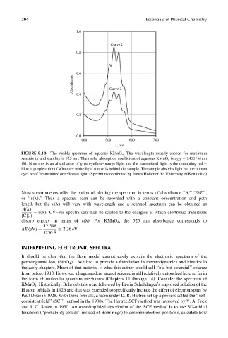
FIGURE 9.10 The visible spectrum of aqueous KMnO 4 . The wavelength usually chosen for maximum
sensitivity and stability is 525 nm. The molar absorption coefficient of aqueous KMnO 4 is e 525 ¼ 2455=Mcm
[8]. Note this is an absorbance of green-yellow-orange light and the transmitted light is the remaining red þ
blue ¼ purple color of whatever white light source is behind the sample. The sample absorbs light but the human
eye ‘‘sees’’ transmitted or reflected light. (Spectrum contributed by James Holler of the University of Kentucky.)

Most spectrometers offer the option of plotting the spectrum in terms of absorbance ‘‘A,’’ ‘‘%T ’’,
or ‘‘e(l).’’ Thus a spectral scan can be recorded with a constant concentration and path
length but the e(l) will vary with wavelength and a scanned spectrum can be obtained as
A(l)
¼ e(l).UV–Vis spectra can then be related to the energies at which electronic transitions
[C](l)
absorb energy in terms of e(l). For KMnO 4 , the 525 nm absorbance corresponds to
12,398
ffi 2:36 eV.
˚
DE (eV) ¼
5250 A
INTERPRETING ELECTRONIC SPECTRA
It should be clear that the Bohr model cannot easily explain the electronic spectrum of the
permanganate ion, (MnO 4 ) . We had to provide a foundation in thermodynamics and kinetics in

the early chapters. Much of that material is what this author would call ‘‘old but essential’’ science
from before 1913. However, a huge modern area of science is still relatively untouched here so far in
the form of molecular quantum mechanics (Chapters 11 through 14). Consider the spectrum of
KMnO 4 . Historically, Bohr orbitals were followed by Erwin Schrödinger’s improved solution of the
H atom orbitals in 1926 and that was extended to specifically include the effect of electron spins by
Paul Dirac in 1928. With these orbitals, a team under D. R. Hartree set up a process called the ‘‘self-
consistent field’’ (SCF) method in the 1930s. The Hartree SCF method was improved by V. A. Fock
and J. C. Slater in 1930. An oversimplified description of the SCF method is to use 3D-orbital
functions (‘‘probability clouds’’ instead of Bohr rings) to describe electron positions, calculate how