Page 113 - Excel Timesaving Techniques for Dummies

22_574272 ch19.qxd 10/1/04 10:41 PM Page 98
98
Technique 19: Controlling When Certain Formats Are Used
Cell Value Is: Compares the value (constant) you 3. Select Less Than in the second drop-down list
specify in the Conditional Formatting dialog box box (the one that now contains Between).
against the value entered in the cell. When Excel
compares this constant to the cell value and the 4. Press Tab to select the last text box and then
criteria you specify for them is met (is between, type 0, as shown in Figure 19-2.
equal to, greater than, less than, greater than or After setting up the condition for the special for-
equal to, or less than or equal to), Excel applies matting, you must specify what formatting attrib-
the conditional formatting to the cell. When the utes to use. The Font attributes that you can set
condition is not met, Excel uses the regular for- for conditional formatting are limited to font
matting applied to the cell. style, underlining, strikethrough, and color. For
Formula Is: Evaluates the logical formula you this example, I turn on strikethrough and bold
enter in the Conditional Formatting dialog box. and select red as the font color.
When this formula evaluates to TRUE, Excel
applies the conditional formatting you define to
the cell. When the formula evaluates to FALSE,
Excel applies the regular formatting to the cell.

When you want to be warned when a cell contains a
particular value or exceeds or falls below a certain
number, the Cell Value Is type of conditional format- • Figure 19-2: The Conditional Formatting dialog box after
ting is the way to go. To get an idea of how you would specifying the first condition.
use this type of conditional formatting, follow along
with the steps for displaying the entry in a cell in red 5. Click the Format button in the Conditional
with bold and strikethrough whenever it contains a Formatting dialog box to open the Format Cells
negative value: dialog box.
6. On the Font, Border, and Patterns tabs, select
1. Position the cell pointer in the cell where you the attributes to be used when the condition is
want to apply conditional formatting. true. When you’re finished selecting your
2. Choose Format➪Conditional Formatting to attributes, click OK. (See Figure 19-3.)
open the Conditional Formatting dialog box, When you close the Format Cells dialog box, the
shown in Figure 19-1. Conditional Formatting dialog box shows your

When Excel opens this dialog box, the Cell Value first condition along with a preview of the for-
Is option is automatically selected along with matting that Excel will apply when the condition
Between as the comparison operator. is true. At this point, you can either add another
condition (see the next section, “When two con-
ditions are better than one”), or if you need only
the one condition — as is the case here — you
can close the dialog box.
7. Click OK to close the Conditional Formatting
dialog box and put the conditional formatting
into effect in the current cell.
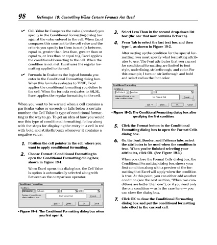
• Figure 19-1: The Conditional Formatting dialog box when
you first open it.