Page 114 - Excel Timesaving Techniques for Dummies

22_574272 ch19.qxd 10/1/04 10:41 PM Page 99
99
Formats to Suit Every Condition
To copy the conditional formatting you see applied
to cell C4 down to the other cells in the Retail Price
column (you don’t want to have to pay to have cus-
tomers take any of your furniture), follow these steps:

1. Copy cell C4 to the Clipboard (Ctrl+C) and then
select the cell range C5:C9.
2. Choose Edit➪Paste Special to open the Paste
Special dialog box.
3. Select the Formats option button and then
click OK.
Excel then pastes the conditional formatting for cell
C4 to all the other Retail Price cells, so they will also
alert you with the same kind of in-your-face formatting
should any errant negative entries come their way.

When two conditions are better than one
• Figure 19-3: Selecting the attributes for the first condition
When setting up conditional formatting for a cell,
in the Format Cells dialog box.
you’re not limited to a single condition. You can set
up several conditions, each with its own unique
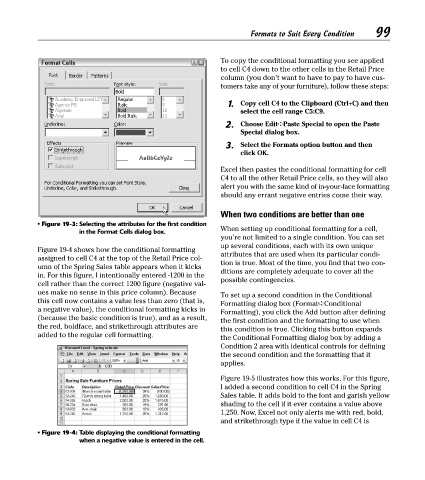
Figure 19-4 shows how the conditional formatting
attributes that are used when its particular condi-
assigned to cell C4 at the top of the Retail Price col-
umn of the Spring Sales table appears when it kicks tion is true. Most of the time, you find that two con-
ditions are completely adequate to cover all the
in. For this figure, I intentionally entered -1200 in the
cell rather than the correct 1200 figure (negative val- possible contingencies.
ues make no sense in this price column). Because To set up a second condition in the Conditional
this cell now contains a value less than zero (that is,
Formatting dialog box (Format➪Conditional
a negative value), the conditional formatting kicks in Formatting), you click the Add button after defining
(because the basic condition is true), and as a result,
the first condition and the formatting to use when
the red, boldface, and strikethrough attributes are this condition is true. Clicking this button expands
added to the regular cell formatting.
the Conditional Formatting dialog box by adding a
Condition 2 area with identical controls for defining
the second condition and the formatting that it
applies.

Figure 19-5 illustrates how this works. For this figure,
I added a second condition to cell C4 in the Spring
Sales table. It adds bold to the font and garish yellow
shading to the cell if it ever contains a value above
1,250. Now, Excel not only alerts me with red, bold,
and strikethrough type if the value in cell C4 is
• Figure 19-4: Table displaying the conditional formatting
when a negative value is entered in the cell.