Page 148 - Finite Element Modeling and Simulations with ANSYS Workbench

Two-Dimensional Elasticity 133

q B
q f
q A f A B
s
B B
A L A

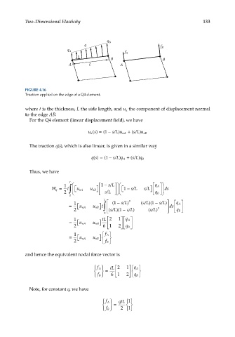
FIGURE 4.16
Traction applied on the edge of a Q4 element.

where t is the thickness, L the side length, and u the component of displacement normal
n
to the edge AB.
For the Q4 element (linear displacement field), we have

us() = ( − sL u nA + / )
1
(
/
)
n s Lu nB
The traction q(s), which is also linear, is given in a similar way
qs() = ( − sL q A + / )
(
1
)
/
s Lq B
Thus, we have
L
sL 
1  1 − /   q A 
W q = t ∫    u nA u nB       1 − / sL    ds
sL
/
/
2   sL    q B 
0
L
/
/
1  1 ( − sL) 2 ( sL 1)(/ − sL)  q A 
∫
=  u nA u nB t   ds  

/
2  ( sL 1)(/ − sL) ( (sL ) 2   q B 
/
0
1 tL 2  1   q A 
=   u nA u nB      
2 6 1 2   q B 

1  f A 
=  u nA u nB   

f
2  B 
and hence the equivalent nodal force vector is
 f A  tL 2 1  q A 
  =    

 f B  6 1 2  q B 
Note, for constant q, we have
 f A  qtL   1
  =  
1
 f B  2  