Page 143 - Finite Element Modeling and Simulations with ANSYS Workbench

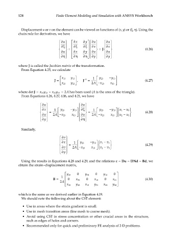
128 Finite Element Modeling and Simulation with ANSYS Workbench

Displacement u or v on the element can be viewed as functions of (x, y) or (ξ, η). Using the
chain rule for derivatives, we have
∂ 
y 
 u  ∂x ∂  ∂u   ∂ u 
      
 ∂ξ  ∂ξ ∂ξ  ∂x   ∂ x 
J
  =     =   (4.26)
y
 ∂u    ∂x ∂  ∂u   ∂ u 


y






 ∂η  ∂η ∂η  ∂ y   ∂ y 
where J is called the Jacobian matrix of the transformation.
From Equation 4.25, we calculate
J = x 13 y 13   , J −1 = 1  y 23 −y 13   (4.27)


x
 23 y 23  2 A  −x 23 x 13 
2
= A has been used (A is the area of the triangle).
23
where det J = xy 23 − xy 13
13
From Equations 4.26, 4.27, 4.16, and 4.21, we have
∂ 
 u  ∂u 

 ∂  1  y 23 −y 13  ∂ξ  1  y − 13  1 u − u 


 x
y

  =     =  23   3  (4.28)
x
 ∂u  2 A  −x 23 x 13   ∂u  2A  − 23 x 13  2 u − u 3 
∂ 
 y  ∂η
    
Similarly,
∂ 
 v

 ∂  1  y 23 −y 13 v 1 − v 3 
 x
  =     (4.29)

 ∂v  2 A  −x 23 x 13  v 2 − v 3 
∂ 
 y
 
Using the results in Equations 4.28 and 4.29, and the relations ε= Du = DNd = Bd, we
obtain the strain–displacement matrix,
y 23 0 y 31 0 y 12 0 
1  
B = 0 x 32 0 x 13 0 x 21 (4.30)
2A   

x 32 y 23 x 13 y 31 x 21 y 12 
which is the same as we derived earlier in Equation 4.19.
We should note the following about the CST element:
• Use in areas where the strain gradient is small.
• Use in mesh transition areas (fine mesh to coarse mesh).
• Avoid using CST in stress concentration or other crucial areas in the structure,
such as edges of holes and corners.
• Recommended only for quick and preliminary FE analysis of 2-D problems.