Page 141 - Finite Element Modeling and Simulations with ANSYS Workbench

126 Finite Element Modeling and Simulation with ANSYS Workbench

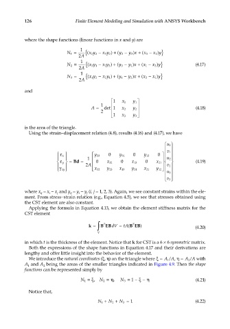
where the shape functions (linear functions in x and y) are

1
N 1 = {( xy 3 − xy 2 + ( y 2 − y x + ( x 3 − xy}
)
3 )
2 )
3
2
2 A
1
−
N 2 = ( { xy 1 − xy 3 + ( y 3 − yx + x 1 − x y } (4.17)
(
)
)
)
3
1
1
3
2 A
1
= ( − xy 1 ) ( − y x ( − xy }
)
)
1
N 3 { xy 2 2 + y 1 2 + x 2 1
2 A
and
1 x 1 y 
1
1  
A = det 1 x 2 y 2 (4.18)
2  

3
1 x 3 y  
is the area of the triangle.
Using the strain–displacement relation (4.8), results (4.16) and (4.17), we have
 1 u 
 
 ε   y 23 0 y 31 0 y 12 0   1 v 
x

  1   2 u 

 ε  = Bd =  0 x 32 0 x 13 0 x 21   (4.19)

y
  2 A  x y   2 v 
 γ xy   x 32 y 23 x 13 y 331 21 12   3 u 
 

  3 v 
where x = x − x and y = y − y (i, j = 1, 2, 3). Again, we see constant strains within the ele-
j
ij
ij
i
i
j
ment. From stress–strain relation (e.g., Equation 4.5), we see that stresses obtained using
the CST element are also constant.
Applying the formula in Equation 4.13, we obtain the element stiffness matrix for the
CST element
T
k = ∫ B EBdV = tA( BEB) (4.20)
T
V
in which t is the thickness of the element. Notice that k for CST is a 6 × 6 symmetric matrix.
Both the expressions of the shape functions in Equation 4.17 and their derivations are
lengthy and offer little insight into the behavior of the element.
/
We introduce the natural coordinates (ξ, η) on the triangle where ξ= AA/ , η= AA with
2
1
A and A being the areas of the smaller triangles indicated in Figure 4.9. Then the shape
2
1
functions can be represented simply by
N 1 =ξ, N 2 =η, N 3 = 1 − ξ− η (4.21)

Notice that,
N 1 + N 2 + N 3 = 1 (4.22)