Page 140 - Finite Element Modeling and Simulations with ANSYS Workbench

Two-Dimensional Elasticity 125

v 3
3
(x , y ) u 3
3
3
v
v 2
v 1 (x, y) u 2
y u 2
1 u (x , y )
2
2
(x , y ) 1
1
1
x
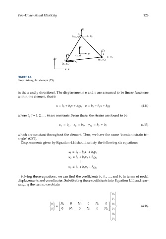
FIGURE 4.8
Linear triangular element (T3).

in the x and y directions). The displacements u and v are assumed to be linear functions
within the element, that is

u = b + bx + by, v = b + bx + by (4.14)
1 2 3 4 5 6

where b (i = 1, 2, …, 6) are constants. From these, the strains are found to be
i
ε= b 2 , ε= b 6 , (4.15)
x y γ xy = b 3 + b 5

which are constant throughout the element. Thus, we have the name “constant strain tri-
angle” (CST).
Displacements given by Equation 4.14 should satisfy the following six equations:

u 1 = b 1 + bx + by
21
31
u 2 = b 1 + bx + by
22
32

v 3 = b 4 + bx + by
53 63
Solving these equations, we can find the coefficients b , b , …, and b in terms of nodal
1
6
2
displacements and coordinates. Substituting these coefficients into Equation 4.14 and rear-
ranging the terms, we obtain
u 
 1
  
 v 1 
 u  N 1 0 N 2 0 N 3 0   u 2 


  =     (4.16)
v
   0 N 1 0 N 2 0 N 3   v 2 
 u 3 
 
  v 3  