Page 242 - Finite Element Modeling and Simulations with ANSYS Workbench

Three-Dimensional Elasticity 227

Whenever possible, one should try to apply higher-order (quadratic) elements, such as
10-node tetrahedron and 20-node brick elements for 3-D stress analysis. Avoid using the
linear, especially the four-node tetrahedron elements in 3-D stress analysis, because they
are inaccurate for such purposes. However, it is fine to use them for deformation analysis
or in vibration analysis (see Chapter 8).

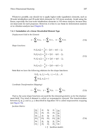
7.4.3 Formulation of a Linear Hexahedral Element Type

Displacement Field in the Element:
8
8
8
u = ∑ N u i , v = ∑ Nv i , w = ∑ N w i (7.11)
i
i
i
i=1 i=1 i=1
Shape Functions:
1
ξη
N 1 (, ,) ζ = 1 ( − ξ )( 1 − η )( 1 − ζ ),
8
1
N 2 (, ,) ζ = 1 ( + ξ )( 1 − η )( 1 − ζ ),
ξη
8 (7.12)
)( +
)( −
N 3 ((, ,)ξη ζ = 1 ( + ξ 1 η 1 ζ ),
1
8

1
ξη
N 8 (, ,) ζ = ( −1 ξ )( +1 η )( +1 ) ζ
8
Note that we have the following relations for the shape functions:
N i (,ξη ζ j ) = δ ij ij, =, 1 , ,… , .
2
8
j ,
j
8
∑ i N (, ,)ξη ζ = 1
i=1
Coordinate Transformation (Mapping):
8
8
8
x = ∑ N x , y = ∑ Ny , z = ∑ N z (7.13)
ii
ii
ii
i=1 i=1 i=1
That is, the same shape functions are used for the element geometry as for the displace-
ment field. This kind of element is called an isoparametric element. The transformation
between (ξ, η, ζ ) and (x, y, z) described by Equation 7.13 is called isoparametric mapping
(see Figure 7.6).
Jacobian Matrix:
 ∂u   ∂x ∂y ∂z   ∂u 
 ∂ξ   ∂ξ ∂ξ ∂ξ   
     ∂x 
 ∂u   ∂x ∂y ∂z   ∂u
  =    
 ∂η   ∂η ∂η ∂η   ∂y  (7.14)
 ∂u   ∂x ∂y ∂z   ∂u 
     
ζ
 ∂ζ   ∂ζ ∂ζ ∂ζ  ∂z 

≡ ≡ J Jacobian matrix