Page 243 - Finite Element Modeling and Simulations with ANSYS Workbench

228 Finite Element Modeling and Simulation with ANSYS Workbench

3
4

8 1 2
7

5 6
x
Mapping (xyz )
(–1≤ , , ≤ 1)

(–1, 1, –1) 4 3 (1, 1, –1)

(–1, 1, 1) 8 7 (1, 1, 1)

o

(–1, –1, –1) 1
2 (1, –1, –1)
(–1, –1, 1) 5 6 (1, –1, 1)

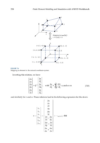
FIGURE 7.6
Mapping an element to the natural coordinate system.
Inverting this relation, we have:

 ∂u   ∂u 
   ∂ξ 
 ∂x     8
 ∂u  −1  ∂u  ∂u ∂N i
  = J   ,with = ∑ u i and so on (7.15)
 ∂y   ∂η  ∂ξ = i 1 ∂ξ
 ∂u   ∂u 

 ∂z   ∂ζ 

 
and similarly for v and w. These relations lead to the following expression for the strain:
 ∂u 
 ∂x 
 
 ∂v 
 ε   ∂y 
x
   
 ε y   ∂w 
 ε   ∂z 


z
ε =   =   = uuse(.615 =Bd
)
u
 γ xy   ∂v + ∂u 
γ  yz   ∂x ∂y 
   ∂w ∂v 
 γ  zx    + 
 ∂y ∂z 
 ∂u ∂w 
 + 
 ∂z ∂x 