Page 97 - Fluid Power Engineering

72 Cha pte r T h ree

Hagen-
64
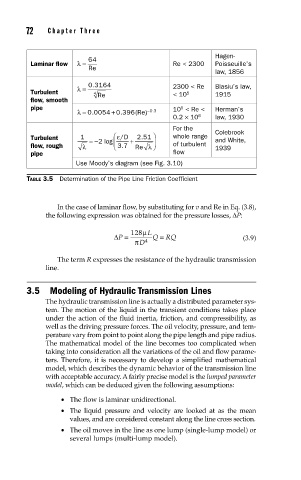
Laminar flow λ= Re < 2300 Poisseuille’s
Re
law, 1856
.
λ= 0 3164 2300 < Re Blasiu’s law,
Turbulent 4 Re < 10 5 1915
flow, smooth
pipe 10 < Re < Herman’s
5
.
λ= 0 0054 0 396. + . (Re) −03
0.2 × 10 6 law, 1930
For the Colebrook
.
Turbulent 1 =− 2 log ε ⎛ /D + 251 ⎞ whole range and White,
flow, rough λ ⎜ ⎝ 37 . Re λ ⎠ ⎟ of turbulent 1939
pipe flow
Use Moody’s diagram (see Fig. 3.10)
TABLE 3.5 Determination of the Pipe Line Friction Coefficient

In the case of laminar flow, by substituting for v and Re in Eq. (3.8),
the following expression was obtained for the pressure losses, ΔP:
128μ L
ΔP = 4 Q = RQ (3.9)
π D
The term R expresses the resistance of the hydraulic transmission
line.

3.5 Modeling of Hydraulic Transmission Lines
The hydraulic transmission line is actually a distributed parameter sys-
tem. The motion of the liquid in the transient conditions takes place
under the action of the fluid inertia, friction, and compressibility, as
well as the driving pressure forces. The oil velocity, pressure, and tem-
perature vary from point to point along the pipe length and pipe radius.
The mathematical model of the line becomes too complicated when
taking into consideration all the variations of the oil and flow parame-
ters. Therefore, it is necessary to develop a simplified mathematical
model, which describes the dynamic behavior of the transmission line
with acceptable accuracy. A fairly precise model is the lumped parameter
model, which can be deduced given the following assumptions:
• The flow is laminar unidirectional.
• The liquid pressure and velocity are looked at as the mean
values, and are considered constant along the line cross section.
• The oil moves in the line as one lump (single-lump model) or
several lumps (multi-lump model).