Page 158 - T. Anderson-Fracture Mechanics - Fundamentals and Applns.-CRC (2005)

1656_C003.fm Page 138 Monday, May 23, 2005 5:42 PM

138 Fracture Mechanics: Fundamentals and Applications

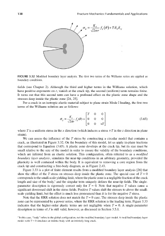
FIGURE 3.32 Modified boundary layer analysis. The first two terms of the Williams series are applied as
boundary conditions.
fields (see Chapter 2). Although the third and higher terms in the Williams solution, which
have positive exponents on r, vanish at the crack tip, the second (uniform) term remains finite.
It turns out that this second term can have a profound effect on the plastic zone shape and the
stresses deep inside the plastic zone [24, 25].
For a crack in an isotropic elastic material subject to plane strain Mode I loading, the first two
terms of the Williams solution are as follows:
T  0 0 
K  
σ = I f () 0 0 0 (3.65)
θ +
ij
2 πr ij  
 0 0 νT 
where T is a uniform stress in the x direction (which induces a stress n T in the z direction in plane
strain).
We can assess the influence of the T stress by constructing a circular model that contains a
crack, as illustrated in Figure 3.32. On the boundary of this model, let us apply in-plane tractions
that correspond to Equation (3.65). A plastic zone develops at the crack tip, but its size must be
small relative to the size of the model in order to ensure the validity of the boundary conditions,
which are inferred from an elastic solution. This configuration, often referred to as a modified
boundary layer analysis, simulates the near-tip conditions in an arbitrary geometry, provided the
plasticity is well contained within the body. It is equivalent to removing a core region from the
crack tip and constructing a free-body diagram, as in Figure 2.43.
Figure 3.33 is a plot of finite element results from a modified boundary layer analysis [26] that
show the effect of the T stress on stresses deep inside the plastic zone. The special case of T = 0
corresponds to the small-scale yielding limit, where the plastic zone is a negligible fraction of the crack
7
length and size of the body, and the singular term uniquely defines the near-tip fields. The single-
parameter description is rigorously correct only for T = 0. Note that negative T values cause a
significant downward shift in the stress fields. Positive T values shift the stresses to above the small-
scale yielding limit, but the effect is much less pronounced than it is for the negative T stress.
Note that the HRR solution does not match the T = 0 case. The stresses deep inside the plastic
zone can be represented by a power series, where the HRR solution is the leading term. Figure 3.33
indicates that the higher-order plastic terms are not negligible when T = 0. A single-parameter
description in terms of J is still valid, however, as discussed in Section 3.5.1.

7 In this case, ‘‘body’’ refers to the global configuration, not the modified boundary layer model. A modified boundary layer
model with T = 0 simulates an infinite body with an infinitely long crack.