Page 159 - T. Anderson-Fracture Mechanics - Fundamentals and Applns.-CRC (2005)

1656_C003.fm Page 139 Monday, May 23, 2005 5:42 PM

Elastic-Plastic Fracture Mechanics 139

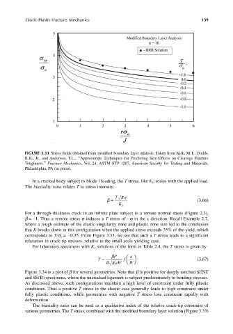
FIGURE 3.33 Stress fields obtained from modified boundary layer analysis. Taken from Kirk, M.T., Dodds,
R.H., Jr., and Anderson, T.L., ‘‘Approximate Techniques for Predicting Size Effects on Cleavage Fracture
Toughness.’’ Fracture Mechanics, Vol. 24, ASTM STP 1207, American Society for Testing and Materials,
Philadelphia, PA (in press).

In a cracked body subject to Mode I loading, the T stress, like K , scales with the applied load.
I
The biaxiality ratio relates T to stress intensity:
T π a
β = (3.66)
K I

For a through-thickness crack in an infinite plate subject to a remote normal stress (Figure 2.3),
b = −1. Thus a remote stress s induces a T stress of –s in the x direction. Recall Example 2.7,
where a rough estimate of the elastic-singularity zone and plastic zone size led to the conclusion
that K breaks down in this configuration when the applied stress exceeds 35% of the yield, which
corresponds to T/s = −0.35. From Figure 3.33, we see that such a T stress leads to a significant
o
relaxation in crack-tip stresses, relative to the small-scale yielding case.
For laboratory specimens with K solutions of the form in Table 2.4, the T stress is given by
I
β P  a 
T = f (3.67)
B a π W  W 
Figure 3.34 is a plot of b for several geometries. Note that b is positive for deeply notched SENT
and SE(B) specimens, where the uncracked ligament is subject predominately to bending stresses.
As discussed above, such configurations maintain a high level of constraint under fully plastic
conditions. Thus a positive T stress in the elastic case generally leads to high constraint under
fully plastic conditions, while geometries with negative T stress lose constraint rapidly with
deformation.
The biaxiality ratio can be used as a qualitative index of the relative crack-tip constraint of
various geometries. The T stress, combined with the modified boundary layer solution (Figure 3.33)