Page 323 - Fundamentals of Gas Shale Reservoirs

INTRODUCTION 303

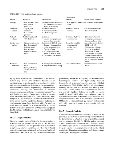
TAbLE 14.1 Tools used to estimate reserves
Conventional
Method Advantage Disadvantage reservoir Unconventional reservoir
Analogy • Best in blanket sands The large number of variables Can be applied in both conventional and unconventional
• Best prior to and parameters causes high assets
production degree of uncertainty
Volumetric • Any stage of Has uncertainties of Accurate in blanket Used only when no wells
method depletion • recovery factor (RF) reservoir have been drilled
• Best prior to • actual drainage area
production
Material Best between 10 and Requires: Accurate in depletion • Should never be used
balance 70% depletion • accurate average pressure drive reservoir • Average pressure cannot
• reservoir fluid properties be measured accurately
Decline curve • Simple, easy to apply Requirements difficult to met Hyperbolic (small b) Must use hyperbolic decline:
analysis • Less data required • Boundary dominated flow or exponential • CBM: b = 0–0.5
(only rate‐time) • Unchanging drainage area decline usually • Shale gas and tight gas:
• Best with long • Fixed skin factor accurate b may be larger than 1
production history • “b” value constant and • Use best‐fit “b” until
• Quick should lie between 0 and 1 predetermined minimum
• Can overestimate reserves decline rate reached, then
impose exponential decline
• Set “b” to proper “terminal
value”
Reservoir • Best with data rich • Needs good history match Used to simulate field Used to simulate individual
simulation wells • Requires much time, costly wells
• In conjunction with
other methods any
time

Spivey, 1996). Reservoir simulation coupled with stochastic published by Warren and Root (1963) and Kazemi (1969).
methods (e.g., Monte Carlo simulation) has provided an Semianalytical solutions for hydraulically fractured
excellent means to predict production profiles for a wide horizontal wells in fractured reservoirs have been published
variety of reservoir characteristics and producing conditions. (Medeiros et al., 2008). PMTx 2.0 (2012), with a number of
The uncertainty is assessed by generating a large number of modeling options, such as a transient dual‐porosity reser-
simulations, sampling from distributions of uncertain voir model (Kazemi, 1969), is an analytical unconventional
geologic, engineering, and other important parameters. This gas reservoir simulator designed to quickly and easily
topic has been an object of study for some time in conven- model single‐well, single‐phase, gas production based on
tional reservoirs (MacMillan et al., 1999; Nakayama, 2000; near‐wellbore reservoir performance under specified well
Sawyer et al., 1999). However, few applications to unconven- completion scenarios. One of the important applications of
tional reservoirs can be found in the literature. Oudinot et al. PMTx 2.0 is to estimate ultimate gas recovery for horizontal
(2005) coupled Monte Carlo simulation with a fractured res- wells with transverse fractures in a rectangular shale gas
ervoir simulator, COMET3, to assess the EUR in coalbed reservoir.
methane reservoirs. Schepers et al. (2009) successfully applied
this Monte Carlo COMET3 procedure to forecast EUR for the 14.1.7 Economic Analysis
Utica Shale.
Almadani (2010) presented a methodology to determine the
percentage of TRR that is economically recoverable from
14.1.6 Analytical Models
the Barnett Shale as a function of gas price and finding and
Given the complex nature of hydraulic fracture growth, the development costs (F&DC). For ERR he applied economic
extremely low permeability of the matrix rock in many criteria of minimum 20% internal rate of return (IRR) and
shale gas reservoirs, and the predominance of horizontal maximum 5‐year payout to recover the initial investment,
completions, reservoir simulation is often the preferred which are hurdles sometimes used by investors in the oil and
method to predict and evaluate well performance. Analytical gas industry. The author suggested that wells that do not pay
solutions for fluid flow in naturally fracture reservoirs were out in 5 years are not good investment.