Page 209 - Fundamentals of Ocean Renewable Energy Generating Electricity From The Sea

198 Fundamentals of Ocean Renewable Energy

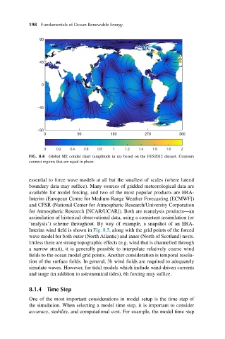
FIG. 8.4 Global M2 cotidal chart (amplitude in m) based on the FES2012 dataset. Contours
connect regions that are equal in phase.

essential to force wave models at all but the smallest of scales (where lateral
boundary data may suffice). Many sources of gridded meteorological data are
available for model forcing, and two of the most popular products are ERA-
Interim (European Centre for Medium Range Weather Forecasting [ECMWF])
and CFSR (National Center for Atmospheric Research/University Corporation
for Atmospheric Research [NCAR/UCAR]). Both are reanalysis products—an
assimilation of historical observational data, using a consistent assimilation (or
‘analysis’) scheme throughout. By way of example, a snapshot of an ERA-
Interim wind field is shown in Fig. 8.5, along with the grid points of the forced
wave model for both outer (North Atlantic) and inner (North of Scotland) nests.
Unless there are strong topographic effects (e.g. wind that is channelled through
a narrow strait), it is generally possible to interpolate relatively coarse wind
fields to the ocean model grid points. Another consideration is temporal resolu-
tion of the surface fields. In general, 3h wind fields are required to adequately
simulate waves. However, for tidal models which include wind-driven currents
and surge (in addition to astronomical tides), 6h forcing may suffice.

8.1.4 Time Step

One of the most important considerations in model setup is the time step of
the simulation. When selecting a model time step, it is important to consider
accuracy, stability, and computational cost. For example, the model time step