Page 212 - Fundamentals of Ocean Renewable Energy Generating Electricity From The Sea

Ocean Modelling for Resource Characterization Chapter | 8 201

u,v u,v v

q q
u u

u,v u,v v
(A) (B)
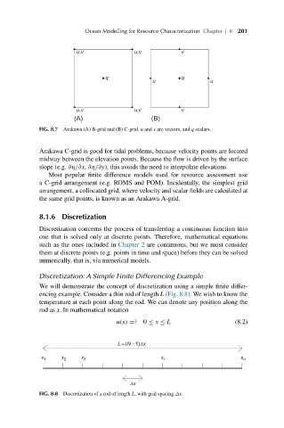
FIG. 8.7 Arakawa (A) B-grid and (B) C-grid. u and v are vectors, and q scalars.

Arakawa C-grid is good for tidal problems, because velocity points are located
midway between the elevation points. Because the flow is driven by the surface
slope (e.g. ∂η/∂x, ∂η/∂y), this avoids the need to interpolate elevations.
Most popular finite difference models used for resource assessment use
a C-grid arrangement (e.g. ROMS and POM). Incidentally, the simplest grid
arrangement, a collocated grid, where velocity and scalar fields are calculated at
the same grid points, is known as an Arakawa A-grid.

8.1.6 Discretization

Discretization concerns the process of transferring a continuous function into
one that is solved only at discrete points. Therefore, mathematical equations
such as the ones included in Chapter 2 are continuous, but we must consider
them at discrete points (e.g. points in time and space) before they can be solved
numerically, that is, via numerical models.

Discretization: A Simple Finite Differencing Example
We will demonstrate the concept of discretization using a simple finite differ-
encing example. Consider a thin rod of length L (Fig. 8.8). We wish to know the
temperature at each point along the rod. We can denote any position along the
rod as x. In mathematical notation
u(x) =? 0 ≤ x ≤ L (8.2)

L= (N − 1)Dx

x 1 x 2 x 3 x i x n

Dx
FIG. 8.8 Discretization of a rod of length L, with grid spacing Δx.