Page 210 - Fundamentals of Ocean Renewable Energy Generating Electricity From The Sea

Ocean Modelling for Resource Characterization Chapter | 8 199

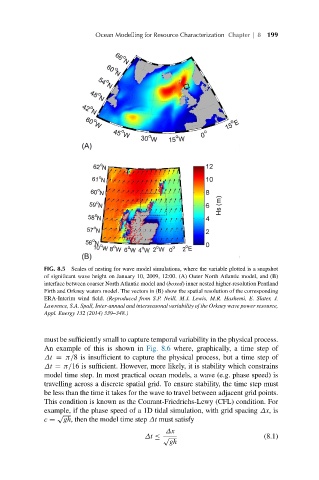
FIG. 8.5 Scales of nesting for wave model simulations, where the variable plotted is a snapshot
of significant wave height on January 10, 2009, 12:00. (A) Outer North Atlantic model, and (B)
interface between coarser North Atlantic model and (boxed) inner nested higher-resolution Pentland
Firth and Orkney waters model. The vectors in (B) show the spatial resolution of the corresponding
ERA-Interim wind field. (Reproduced from S.P. Neill, M.J. Lewis, M.R. Hashemi, E. Slater, J.
Lawrence, S.A. Spall, Inter-annual and interseasonal variability of the Orkney wave power resource,
Appl. Energy 132 (2014) 339–348.)

must be sufficiently small to capture temporal variability in the physical process.
An example of this is shown in Fig. 8.6 where, graphically, a time step of
Δt = π/8 is insufficient to capture the physical process, but a time step of
Δt = π/16 is sufficient. However, more likely, it is stability which constrains
model time step. In most practical ocean models, a wave (e.g. phase speed) is
travelling across a discrete spatial grid. To ensure stability, the time step must
be less than the time it takes for the wave to travel between adjacent grid points.
This condition is known as the Courant-Friedrichs-Lewy (CFL) condition. For
example, if the phase speed of a 1D tidal simulation, with grid spacing Δx,is
√
c = gh, then the model time step Δt must satisfy
Δx
Δt ≤ √ (8.1)
gh