Page 211 - Fundamentals of Ocean Renewable Energy Generating Electricity From The Sea

200 Fundamentals of Ocean Renewable Energy

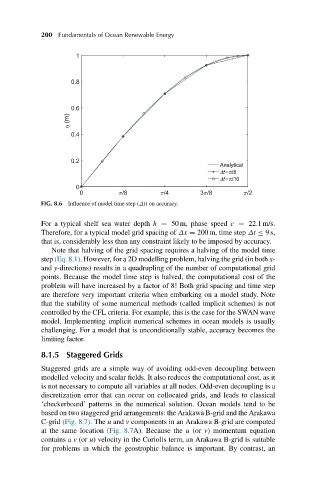
FIG. 8.6 Influence of model time step (Δt) on accuracy.

For a typical shelf sea water depth h = 50 m, phase speed c = 22.1 m/s.
Therefore, for a typical model grid spacing of Δx = 200 m, time step Δt ≤ 9s,
that is, considerably less than any constraint likely to be imposed by accuracy.
Note that halving of the grid spacing requires a halving of the model time
step (Eq. 8.1). However, for a 2D modelling problem, halving the grid (in both x-
and y-directions) results in a quadrupling of the number of computational grid
points. Because the model time step is halved, the computational cost of the
problem will have increased by a factor of 8! Both grid spacing and time step
are therefore very important criteria when embarking on a model study. Note
that the stability of some numerical methods (called implicit schemes) is not
controlled by the CFL criteria. For example, this is the case for the SWAN wave
model. Implementing implicit numerical schemes in ocean models is usually
challenging. For a model that is unconditionally stable, accuracy becomes the
limiting factor.
8.1.5 Staggered Grids

Staggered grids are a simple way of avoiding odd-even decoupling between
modelled velocity and scalar fields. It also reduces the computational cost, as it
is not necessary to compute all variables at all nodes. Odd-even decoupling is a
discretization error that can occur on collocated grids, and leads to classical
‘checkerboard’ patterns in the numerical solution. Ocean models tend to be
based on two staggered grid arrangements: the Arakawa B-grid and the Arakawa
C-grid (Fig. 8.7). The u and v components in an Arakawa B-grid are computed
at the same location (Fig. 8.7A). Because the u (or v) momentum equation
contains a v (or u) velocity in the Coriolis term, an Arakawa B-grid is suitable
for problems in which the geostrophic balance is important. By contrast, an