Page 82 - Fundamentals of Probability and Statistics for Engineers

Random Variables and Probability Distributions 65
Consider now the conditional mass function p XY (x y). With Y ˆ y having
j
happened, the situation is again similar to that for determining p (y) except
Y
that the number of cars available for taking possible eastward turns is now
n y; also, here, the probabilities p and r need to be renormalized so that they
sum to 1. Hence, p XY (x y) takes the form
j
x
n y x
n y p p

p xjy†ˆ 1 ; x ˆ 0;1;...;n y; y ˆ 0;1;...;n:
XY
x r ‡ p r ‡ p
3:52†
Finally, we have p XY (x, y) as the product of the two expressions given by
Equations (3.51) and (3.52). The ranges of values for x and y are x ˆ 0, 1, .. . ,
n y, and y ˆ 0, 1,..., n.
Note that p (x, y) has a rather complicated expression that could not have
XY
been derived easily in a direct way. This also points out the need to exercise care
in determining the limits of validity for x and y.

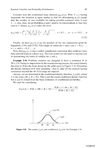
Example 3.10. Problem: resistors are designed to have a resistance R of
2 . Owing to imprecision in the manufacturing process, the actual density
50
function of R has the form shown by the solid curve in Figure 3.18. Determine
the density function of R after screening – that is, after all the resistors having
resistances beyond the 48–52
range are rejected.
Answer: we are interested in the conditional density function, f (r A), where
R j
A is the event f48 R 52g . This is not the usual conditional density function
but it can be found from the basic definition of conditional probability.
We start by considering
P R r \ 48 R 52†
F R rjA†ˆ P R rj48 R 52†ˆ :
P 48 R 52†

f R

f (r\A)
R

f (r)
R
r(Ω)
48 50 52

Figure 3.18 The actual, f (r), and conditional, f (r A), for Example 3.10
j
R
R

TLFeBOOK