Page 401 - Fundamentals of Radar Signal Processing

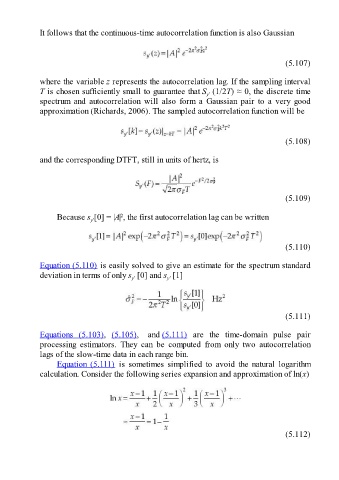
It follows that the continuous-time autocorrelation function is also Gaussian

(5.107)

where the variable z represents the autocorrelation lag. If the sampling interval
T is chosen sufficiently small to guarantee that S (1/2T) ≈ 0, the discrete time
y′
spectrum and autocorrelation will also form a Gaussian pair to a very good
approximation (Richards, 2006). The sampled autocorrelation function will be

(5.108)

and the corresponding DTFT, still in units of hertz, is

(5.109)

Because s [0] = |A| , the first autocorrelation lag can be written
2
y′

(5.110)

Equation (5.110) is easily solved to give an estimate for the spectrum standard
deviation in terms of only s [0] and s [1]
y′
y′

(5.111)

Equations (5.103), (5.105), and (5.111) are the time-domain pulse pair
processing estimators. They can be computed from only two autocorrelation
lags of the slow-time data in each range bin.
Equation (5.111) is sometimes simplified to avoid the natural logarithm
calculation. Consider the following series expansion and approximation of ln(x)

(5.112)