Page 400 - Fundamentals of Radar Signal Processing

spectrum of a finite segment would then be an asinc function squared. Now

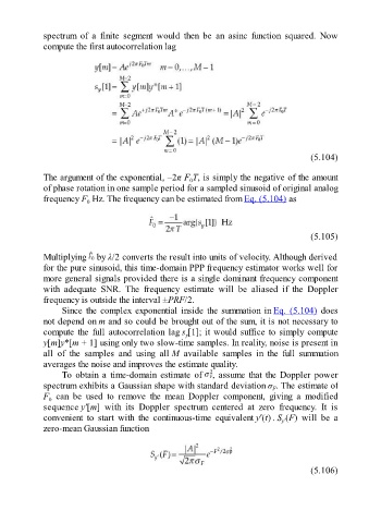
compute the first autocorrelation lag

(5.104)

The argument of the exponential, –2π F T, is simply the negative of the amount
0
of phase rotation in one sample period for a sampled sinusoid of original analog
frequency F Hz. The frequency can be estimated from Eq. (5.104) as
0

(5.105)

Multiplying by λ/2 converts the result into units of velocity. Although derived
for the pure sinusoid, this time-domain PPP frequency estimator works well for
more general signals provided there is a single dominant frequency component

with adequate SNR. The frequency estimate will be aliased if the Doppler
frequency is outside the interval ±PRF/2.
Since the complex exponential inside the summation in Eq. (5.104) does
not depend on m and so could be brought out of the sum, it is not necessary to
compute the full autocorrelation lag s [1]; it would suffice to simply compute
y
y[m]y*[m + 1] using only two slow-time samples. In reality, noise is present in
all of the samples and using all M available samples in the full summation
averages the noise and improves the estimate quality.

To obtain a time-domain estimate of , assume that the Doppler power
spectrum exhibits a Gaussian shape with standard deviation σ . The estimate of
F
F can be used to remove the mean Doppler component, giving a modified
0
sequence y′[m] with its Doppler spectrum centered at zero frequency. It is
convenient to start with the continuous-time equivalent y′(t) . S (F) will be a
y′
zero-mean Gaussian function

(5.106)