Page 426 - Fundamentals of Radar Signal Processing

m/s and T = 2 ms, then M = 3.75 pulses. A typical DPCA implementation will
s
round M to the nearest integer for coarse alignment of the two data streams and
s
then use adaptive processing as described next to achieve good clutter
cancellation.

5.7.2 Adaptive DPCA
While conventional bandlimited interpolation could be used to implement
fractional-PRI timing adjustments, in practice there will also be mismatches

between channels that will make it impossible to achieve high cancellation
ratios even if the time alignment is perfect. Adaptive processing can be
combined with the basic DPCA cancellation to minimize the clutter residue at
the processor output and therefore maximize the improvement factor. The
following discussion of adaptive DPCA is modeled after the “suboptimum
matched filter algorithm” in Shaw and McAulay (1983). This algorithm assumes
that an integer PRI delay of one channel with respect to the other is used to

achieve coarse time alignment of the two-phase center channels to be combined.
Each received signal channel is then divided into Doppler bins using a DFT.
MTI cancellation is performed independently in each subband, allowing the
adaptive cancellation weight to be optimized separately for each Doppler bin
and improving overall performance.
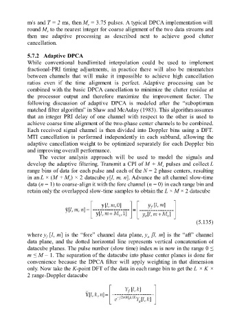
The vector analysis approach will be used to model the signals and

develop the adaptive filtering. Transmit a CPI of M + M pulses and collect L
s
range bins of data for each pulse and each of the N = 2 phase centers, resulting
in an L × (M + M ) × 2 datacube y[l, m, n]. Advance the aft channel slow-time
s
data (n = 1) to coarse-align it with the fore channel (n = 0) in each range bin and
retain only the overlapped slow-time samples to obtain the L × M × 2 datacube

(5.135)

where y [l, m] is the “fore” channel data plane, y [l, m] is the “aft” channel
f
a
data plane, and the dotted horizontal line represents vertical concatenation of
datacube planes. The pulse number (slow time) index m is now in the range 0 ≤

m ≤ M – 1. The separation of the datacube into phase center planes is done for
convenience because the DPCA filter will apply weighting in that dimension
only. Now take the K-point DFT of the data in each range bin to get the L × K ×
2 range-Doppler datacube