Page 274 - Fundamentals of Reservoir Engineering

OILWELL TESTING 211

5
The original paper on the subject was presented by Odeh and Jones in which the
analysis technique is precisely as described above except that the p functions in
D
equ. (7.69) were evaluated for transient flow as

4t
p D () = 1 2 ln D (7.23)
t
D
γ
This leads to the test analysis equation (with t in hours)

p −
kh ( i p wf ) n ∆ q j k
7.08 10 − 3 n = 1.151 log t − t j 1 ) log 2 − 3.23 0.87S
×
+
+
( n
−
µ B o q n j1 q n φµ cr w
=
(7.72)
which, providing the assumption of transient flow is appropriate for the test, will give a
linear plot of (p i−p wf)/q n versus Σ ∆q j/q n log(t n−t j-1), with slope m = 162.6µB o/kh and
2
intercept m(log(k/φµcr ) −3.23 + .87S), from which k and S can be calculated.
w
It is frequently stated in the literature that the separate flow periods should be of short
duration so that transient flow conditions will prevail at each rate. While this condition is
necessary, it is insufficient for the valid application of transient analysis to the test.
Instead, the entire test, from start to finish, should be sufficiently short so that
transience is assured throughout the whole test period. The reason for this restriction is
that the largest value of the dimensionless time argument, for which the p D functions in
equ. (7.69) must be evaluated, is equal to the total duration of the test. This point is
illustrated in fig. 7.27 (b), which again demonstrates the basic principle of superposition
and shows that in evaluating the flowing pressure at the very end of the test there is
still a component of the pressure response due to the first flow rate to be included in
the superposed constant terminal rate solution. The following example will illustrate the
magnitude of the error that can be made by automatically assuming that a multi-rate
flow test can be interpreted using transient analysis techniques.

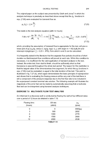
EXERCISE 7.8 MULTI-RATE FLOW TEST ANALYSIS

An initial test in a discovery well is conducted by flowing the well at four different rates
over a period of 12 hours as detailed in table 7.10.

Flowing time Oil rate p wf
(hours) (stb/d) (psia)

0 0 3000(p i)
3 500 2892
6 1000 2778
9 1500 2660
12 2000 2538
TABLE 7.10