Page 273 - Fundamentals of Reservoir Engineering

OILWELL TESTING 210

Conventionally in the analysis of such a test the pressures p, p , . . . are read
wf
wf
2
1
from the pressure chart at the end of each separate flow period and matched to the
theoretical equation (7.69). For instance, the calculation of p wf 3 at the end of the third
flow period is

p −
3 kh ( i p wf 3 ) ( 1 ) 0 (q − q )
q −
7.08 10 − = p D ( ) + 2 1 p D ( D − t D )
t
t
×
D
µ B o q 3 q 3 3 q3 3 1 (7.70)
(q + q 2 )
3
t
+ p ( D − t ) + S
q 3 D 3 D 2
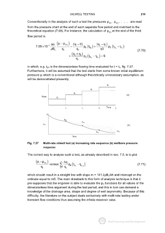
in which, e.g. t D3 is the dimensionless flowing time evaluated for t = t 3, fig. 7.27.
Furthermore, it will be assumed that the test starts from some known initial equilibrium
pressure p i which is a conventional although theoretically unnecessary assumption, as
will be demonstrated presently.
q 4
q 3
q 2
(a)
Rate
q 1

Time
t 1 t 2 t 3 t 4

p i
p wf 1
p wf 2
(b)
p wf
p wf 4
p wf 3
Time

Fig. 7.27 Multi-rate oilwell test (a) increasing rate sequence (b) wellbore pressure
response

The correct way to analyse such a test, as already described in sec. 7.5, is to plot

p − p ) n q
( i wf n versus ∆ j p t − t ) (7.71)
q n j1 q n D ( D n D − j 1
=

which should result in a straight line with slope m = 141.2µB o/kh and intercept on the
ordinate equal to mS. The main drawback to this form of analysis technique is that it
pre-supposes that the engineer is able to evaluate the p D functions for all values of the
dimensionless time argument during the test period, and this in turn can demand a
knowledge of the drainage area, shape and degree of well asymmetry. Because of this
difficulty, the literature on the subject deals exclusively with multi-rate testing under
transient flow conditions thus assuming the infinite reservoir case.