Page 276 - Fundamentals of Reservoir Engineering

OILWELL TESTING 213

2 4
1 1

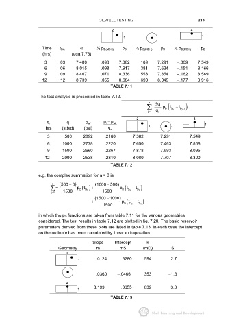
Time t DA α ½ p D(MBH) p D ½ p D(MBH) p D ½ p D(MBH) p D
(hrs) (equ.7.73)

3 .03 7.480 .098 7.382 .189 7.291 −.069 7.549
6 .06 8.015 .098 7.917 .381 7.634 −.151 8.166
9 .09 8.407 .071 8.336 .553 7.854 −.162 8.569
12 .12 8.739 .055 8.684 .690 8.049 −.177 8.916
TABLE 7.11

The test analysis is presented in table 7.12.
n ∆ q
i p D ( D n t D j 1 )
t −
j1 q n −
=
2 4
i
t n q p wf p − p wf 1
hrs (stb/d) (psi) q n 1
3 500 2892 .2160 7.382 7.291 7.549
6 1000 2778 .2220 7.650 7.463 7.858
9 1500 2660 .2267 7.878 7.593 8.095

12 2000 2538 .2310 8.080 7.707 8.300
TABLE 7.12

e.g. the complex summation for n = 3 is

3 (500 0− ) (1000 500− )
t
t
= p D ( ) + p D ( D 9 − t D 3 )
D
9
j1 1500 1500
=
(1500 1000− )
t
+ p D ( D − t D )
1500 9 6
in which the p D functions are taken from table 7.11 for the various geometries
considered. The test results in table 7.12 are plotted in fig. 7.28. The basic reservoir
parameters derived from these plots are listed in table 7.13. In each case the intercept
on the ordinate has been calculated by linear extrapolation.

Slope Intercept k
Geometry m mS (mD) S
2
.0124 .5280 594 2.7
1

.0360 −.0466 353 −1.3

4
1 0.199 .0655 639 3.3
TABLE 7.13