Page 342 - Fundamentals of Water Treatment Unit Processes : Physical, Chemical, and Biological

Flocculation 297

d j i
i j
j

Particle Collision Particle
outside trajectory outside
Collision
trajectory shadow trajectory trajectory
shadow shadow
shadow
d i
Critical
distance Critical
d +d j x c distance
i
(a) (b)
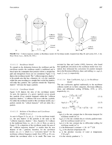
FIGURE 11.2 Collision trajectory models. (a) Rectilinear model. (b) Curvilinear model. (Adapted from Han, M. and Lawler, D.F., J. Am.
Water Works Assoc., 84(10), 80, 1992.)

11.4.1.1.3 Rectilinear Model revisited by Han and Lawler (1992), however, who found
To expand on the distinction between the rectilinear and the that significant corrections to the rectilinear model were war-
curvilinear models, the rectilinear model is traditional and is ranted; they delineated the corrections for particle transport
based upon the assumption that particles follow a straight-line due to the Brownian diffusion, shear, and settling, i.e., a B (i, j),
path and interparticle forces are not considered. Figure 11.2a a SH (i, j), a S (i, j), respectively.
depicts the rectilinear model. The ‘‘collision trajectory shadow’’
is the pseudo area that has a diameter, (d i þ d j ); the i particles
11.4.1.1.6 Rate Coefficients, k B (i, j), for Rectilinear
within this area traveling in a straight line toward the particle j
will strike the j particle. The i particles outside the ‘‘trajectory Model
shadow’’ will miss the larger j particle. The rate coefficients applied traditionally to the rectilinear
collision model are in three categories, Brownian diffusion,
11.4.1.1.4 Curvilinear Model shear, and differential settling (O’Melia, 1978, p. 227),
respectively, i.e.,
Figure 11.2b depicts the idea of the curvilinear model.
As seen, the trajectory of a given i particle curves around 2
2 kT abs (d i þ d j )
the j particle. If an i particle originates within the ‘‘collision (11:4)
k B (i, j) ¼
trajectory shadow,’’ a collision will occur with the j particle. 3 m d i d j
For either the rectilinear model or the curvilinear model, any i (d i þ d j ) 3
particle outside the ‘‘critical diameter’’ will not strike the j k SH (i, j) ¼ G (11:5)
6
particle.
pg(SG p 1) 3
(d i þ d j ) (d i d j ) (11:6)
72n
k S (i, j) ¼
11.4.1.1.5 Relation of Rectilinear and Curvilinear where
Models to a(i, j) k B (i, j) is the rate constant due to Brownian transport for
3
As seen in Figure 11.2a, a(i, j) ¼ 1 for the rectilinear model, rectilinear model (m =s)
i.e., the area shadow of the particles is the same as the k SH (i, j) is the rate constant due to velocity gradient trans-
3
‘‘collision trajectory shadow.’’ Also, Equation 11.1 reduces port for rectilinear model (m =s)
to the traditional form, i.e., g(i, j) ¼ k(i, j). Next, as seen in k S (i, j) is the rate constant due to differential settling for
3
Figure 11.2b, a depiction of the curvilinear model, the area of rectilinear model (m =s)
the ‘‘collision trajectory shadow’’ is smaller than the area k is the Boltzmann’s constant ¼ 1.38 10 23 J=K
shadow of the i particles; therefore, for the curvilinear T abs is the absolute temperature (K)
model, a(i, j) < 1, which is a ‘‘correction factor’’ for the m is the absolute viscosity of water at temperature,
2
rectilinear collision frequency model. Ives (1978, p. 45) con- T (N s=m )
1
sidered the curvilinear effect to be small. The issue was G is the velocity gradient (s )